Why Deep Learning?
- Time
- ~102 min
- Sections
- 13
- Code cells
- 35
- Labs
- 7
- Figures
- 11
Before you start
Deep learning is not "a stronger model". The one real change is that the description of each example is learned from data instead of written by you. This lesson shows the idea with three experiments: a straight-line model that cannot solve a spiral, a hand-made fix that can, and a small network that finds that fix on its own. Then comes an honest counter-example where deep learning buys you nothing.
- Goal
Understand what genuinely changes when a model learns its own representations instead of consuming features that you engineered by hand.
- Outcome
By the end of this lesson you can state precisely what deep learning buys you — and, just as importantly, name the situations where it buys you nothing at all. You will have seen both cases with your own data and your own numbers.
- You will be able to
- explain why neural networks exist, in terms of the ML pipeline you already know;
- distinguish a learned parameter from an engineered feature;
- describe the classical ML pipeline and the deep learning pipeline, and identify exactly where they diverge;
- identify problem types where classical ML remains the correct professional choice in 2026;
- explain why raw pixels and raw text defeat manual feature engineering;
- state where feature engineering still lives inside modern deep learning.
Setup — imports, versions and device detection used by the notebook (2 cells)
Run this once. Everything in this lesson is CPU-only, but we check for an accelerator now because Lessons 1.2 and 1.3 will use one if it exists.
pip install torchRequirement already satisfied: torch in /opt/anaconda3/lib/python3.13/site-packages (2.14.0) Requirement already satisfied: filelock in /opt/anaconda3/lib/python3.13/site-packages (from torch) (3.20.0) Requirement already satisfied: typing-extensions>=4.10.0 in /opt/anaconda3/lib/python3.13/site-packages (from torch) (4.15.0) Requirement already satisfied: setuptools>=77.0.3 in /opt/anaconda3/lib/python3.13/site-packages (from torch) (80.9.0) Requirement already satisfied: sympy>=1.13.3 in /opt/anaconda3/lib/python3.13/site-packages (from torch) (1.14.0) Requirement already satisfied: networkx>=2.5.1 in /opt/anaconda3/lib/python3.13/site-packages (from torch) (3.5) Requirement already satisfied: jinja2 in /opt/anaconda3/lib/python3.13/site-packages (from torch) (3.1.5) Requirement already satisfied: fsspec>=0.8.5 in /opt/anaconda3/lib/python3.13/site-packages (from torch) (2025.10.0) Requirement already satisfied: mpmath<1.4,>=1.1.0 in /opt/anaconda3/lib/python3.13/site-packages (from sympy>=1.13.3->torch) (1.3.0) Requirement already satisfied: MarkupSafe>=2.0 in /opt/anaconda3/lib/python3.13/site-packages (from jinja2->torch) (3.0.2) Note: you may need to restart the kernel to use updated packages.
# Pinned for reproducibility. If a version differs on your machine, the code still runs,# but numbers may shift slightly in the last decimal place.# numpy>=2.0 pandas>=2.2 scikit-learn>=1.5 matplotlib>=3.8 torch>=2.4import sys, warningsimport numpy as npimport pandas as pdimport matplotlib.pyplot as pltimport sklearnwarnings.filterwarnings("ignore")SEED = 42np.random.seed(SEED)print(f"python {sys.version.split()[0]}")print(f"numpy {np.__version__}")print(f"pandas {pd.__version__}")print(f"scikit-learn {sklearn.__version__}")# --- accelerator detection (used from Lesson 1.3 onward) ---try: import torch if torch.cuda.is_available(): DEVICE = "cuda" elif torch.backends.mps.is_available(): DEVICE = "mps" else: DEVICE = "cpu" print(f"torch {torch.__version__} -> device: {DEVICE}")except ImportError: DEVICE = "cpu" print("torch not installed yet (needed from Note 1.3)")python 3.13.9 numpy 2.3.5 pandas 2.3.3 scikit-learn 1.7.2 torch 2.14.0 -> device: mps
Where we are in the course
You arrive at this course already able to do a great deal. You can load a messy dataset, clean it, explore it, encode categoricals, split it properly, fit a model, tune it, and evaluate it honestly. That is not a small skill set. Most of what follows depends on it.
So it is worth being precise about what is actually new here, because the honest answer is narrower than the marketing suggests.
In everything you have built so far, you decided what the model would look at. You chose the columns. You created the ratios, the log transforms, the interaction terms, the aggregations over time windows. The learning algorithm optimised coefficients or split points, but the description of each example — the thing the algorithm actually consumed — came from your judgement.
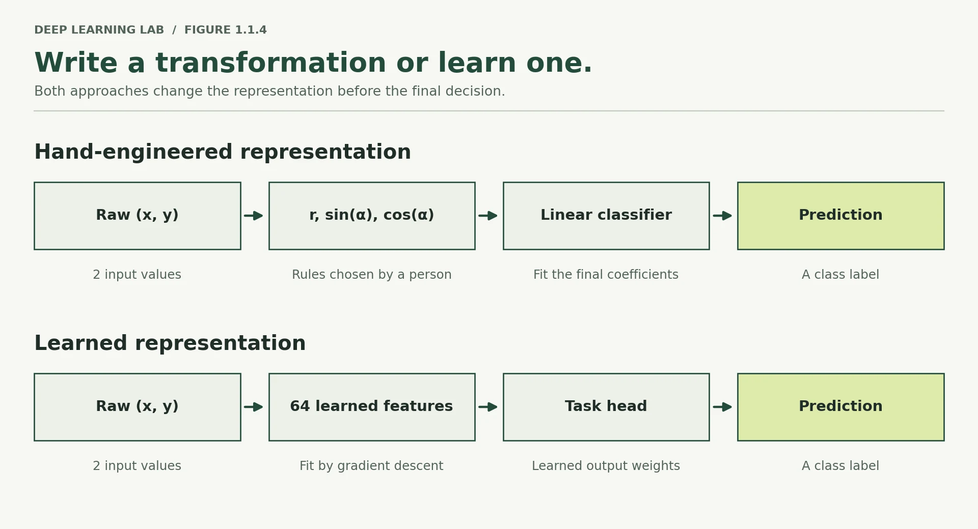
Deep learning moves that description inside the model. The network is handed something closer to the raw signal and learns, as part of the same optimisation that fits the final prediction, what the useful intermediate descriptions are.
That single shift is what this entire course is built on, and it is what makes foundation models possible. Here is the road ahead:
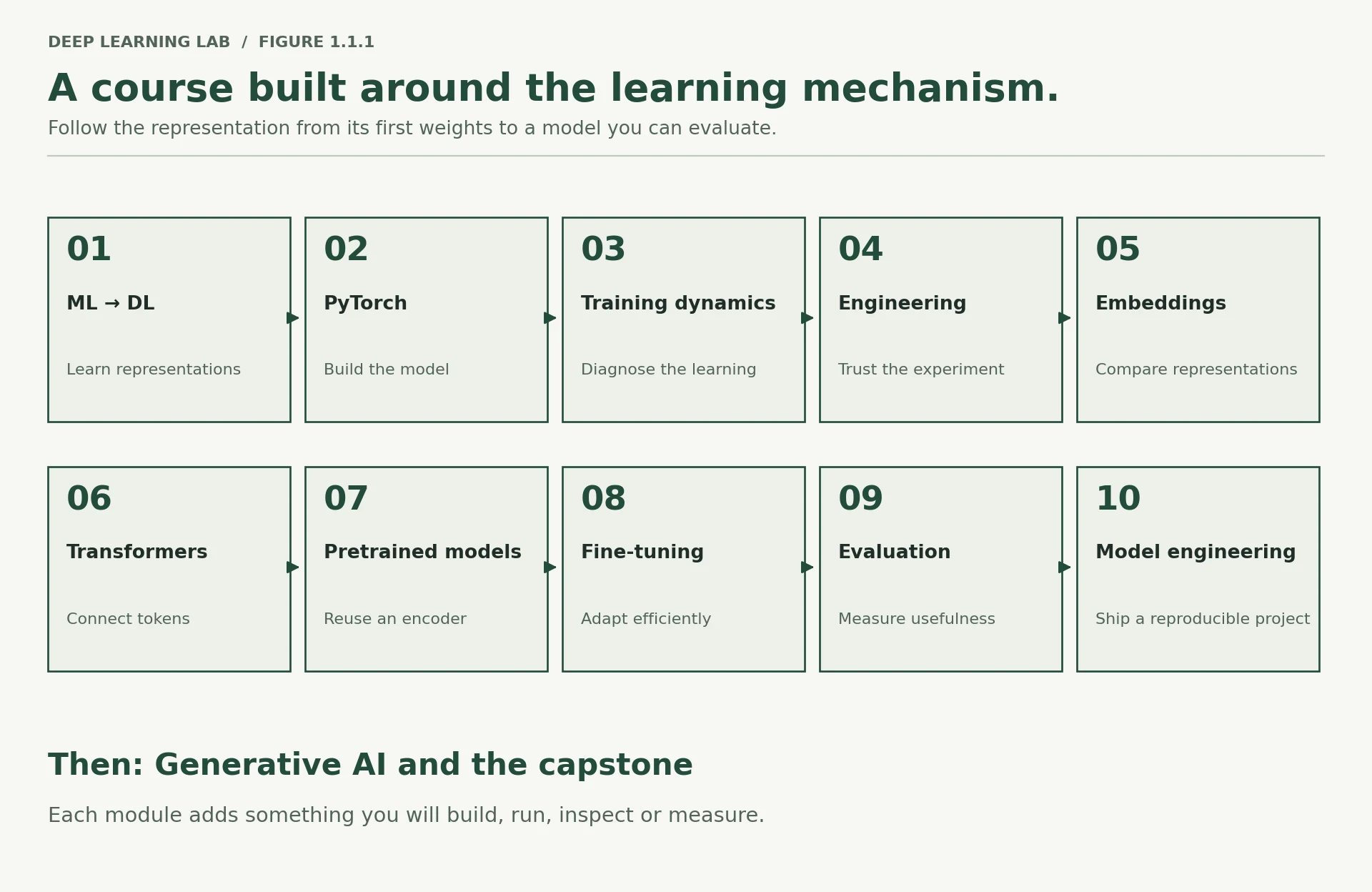
You are at the far left. By Module 10 you will be at the far right, and each arrow will be something you have actually run.
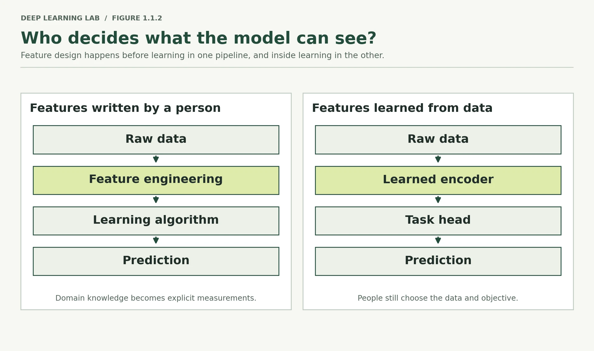
In classical ML the data is transformed once, by hand (the colour change at feature engineering). In deep learning it is transformed gradually, by layers whose weights are learned (the smooth colour shift).
-
Name one feature you engineered in a past project that took real domain knowledge to invent. Could a model plausibly have discovered it from raw data? What would it have needed in order to do so?
Example answer. In a churn project I created “number of support calls in the last 30 days divided by tenure”. It took domain knowledge: the business knew that frustrated new customers leave fastest.
Could a model discover it? Only if two things were true: (1) it saw the raw events (the individual support calls with timestamps) rather than an already-summarised table, and (2) it had enough examples to find the pattern by itself. A network fed the raw event log could learn "recent calls matter more for new customers", but it would need far more data than you needed to write the feature. That trade, your knowledge versus the model's data, runs through this whole lesson.
According to this lesson, what is the one genuinely new thing deep learning brings to someone who already does classical ML well?
Classical ML optimises coefficients or split points on columns you chose. Deep learning moves the choice of the description (the features) inside the model, fitted jointly with the prediction.
Explain, in two sentences, who decides what the model looks at in classical ML, and who decides it in deep learning.
- In classical ML a person chooses and builds the features (columns, ratios, interactions); the algorithm only fits weights or splits on them.
- In deep learning the network learns its own intermediate descriptions from rawer input, as part of the same training that fits the prediction.
A problem your current toolkit should handle
Rather than argue about pipelines in the abstract, let us construct a problem where the difference becomes visible in a single plot.
The problem is deliberately tiny: two features, two classes, one thousand points. There is no missing data, no leakage, no class imbalance, no categorical encoding to worry about. Every complication you normally spend your time on has been removed. Only the shape of the decision boundary remains.
That is the point. When a model fails here, there is nowhere to hide.
def make_spirals(n_per_class=500, noise=0.04, revolutions=2.5, seed=SEED): """Generate two interleaved spiral arms, one per class. A spiral is a circle whose radius grows as you go round it. Each point is placed at a random distance ``t`` along its arm; the radius grows from 0 at the centre to 1 at the outer end while the angle winds ``revolutions`` times. Class 1 is class 0 rotated by half a turn, so its arm sits exactly between the turns of the other. Args: n_per_class: Number of points generated for each of the two classes. noise: Standard deviation of the Gaussian noise added to both coordinates. 0 gives perfectly thin arms; larger values blur the arms into each other. revolutions: How many full turns each arm makes. seed: Seed for the random generator, so the same arguments always give exactly the same dataset. Returns: A tuple ``(X, y)`` where ``X`` is a float array of shape ``(2 * n_per_class, 2)`` holding the (x1, x2) coordinates and ``y`` is an int array of shape ``(2 * n_per_class,)`` holding class labels 0 or 1. Rows are shuffled, so the two classes are mixed. """ rng = np.random.default_rng(seed) Xs, ys = [], [] for c in range(2): # sqrt() spreads points evenly over area rather than bunching them at the centre t = np.sqrt(rng.random(n_per_class)) * revolutions * 2 * np.pi r = t / (revolutions * 2 * np.pi) # radius grows from 0 to 1 theta = t + c * np.pi # second arm is rotated half a turn x1 = r * np.cos(theta) + rng.normal(0, noise, n_per_class) x2 = r * np.sin(theta) + rng.normal(0, noise, n_per_class) Xs.append(np.stack([x1, x2], axis=1)) ys.append(np.full(n_per_class, c)) X = np.vstack(Xs) y = np.concatenate(ys) perm = rng.permutation(len(y)) return X[perm], y[perm]REVOLUTIONS = 2.5X, y = make_spirals(revolutions=REVOLUTIONS)print("X shape:", X.shape, " y shape:", y.shape, " class balance:", np.bincount(y))Builds the dataset: two spiral arms, 500 points each, with a little noise. It uses the idea that a spiral is a circle whose radius grows as you go round it.
- 1
A seeded random generator: the same seed gives exactly the same dataset every time (reproducibility).
- 2
tis how far along the arm each point is, in radians. The square root spreads points evenly by area, so the centre isn't overcrowded. - 3
Radius grows in proportion to
t, from 0 at the centre to 1 at the outer end. This is what makes it a spiral. - 4
The angle. Class 1 (
c = 1) is rotated by π (half a turn), so its arm sits between the turns of class 0's arm. - 5
Polar → Cartesian: \(x_1 = r\cos\theta\), \(x_2 = r\sin\theta\), plus Gaussian noise with standard deviation
noise. - 6
Shuffles the rows so the two classes are mixed together. Good practice before any splitting.
X shape: (1000, 2) y shape: (1000,) class balance: [500 500]
fig, ax = plt.subplots(figsize=(5.5, 5.5))ax.scatter(X[y == 0, 0], X[y == 0, 1], s=8, c="#3b6ea5", label="class 0")ax.scatter(X[y == 1, 0], X[y == 1, 1], s=8, c="#d1701c", label="class 1")ax.set_title("Two spirals — perfectly clean, perfectly labelled")ax.set_xlabel("x1"); ax.set_ylabel("x2"); ax.legend(); ax.set_aspect("equal")plt.tight_layout(); plt.show()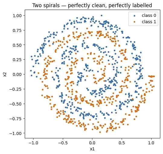
Look at it for a moment before moving on. A human sees the structure instantly. The two arms are obvious, the rule separating them is obvious, and you could label a new point by eye without hesitation.
Hold onto that, because the model is about to fail at something you can do effortlessly.
-
If you had to describe the separating rule in words to a colleague, what would you say? Notice that your description almost certainly involves distance from the centre and angle, not x1 and x2 directly. Remember that — it becomes important in Section 4.
Something like: “Walk out from the centre. The label depends on which arm you are on. Each arm is a band that winds around, so what matters is how far out you are together with which direction you're facing.”
That rule is about distance (radius) and direction (angle), not about \(x_1\) or \(x_2\) on their own. You automatically described the data in a different coordinate system, and that is exactly the insight Section 4 turns into code.
Why is the spiral problem deliberately stripped of missing data, leakage, imbalance and categorical columns?
With every usual complication removed, a failure can only mean the model cannot express the boundary. That makes the diagnosis unambiguous.
Two spirals, and a linear model that cannot
A logistic regression draws exactly one straight line through your feature space. Every point on one side receives one label, every point on the other side receives the other. That constraint is not a weakness in the implementation, not a bug, and not something a better optimiser would fix. It is the definition of the model.
Now look again at what we are asking it to separate. Walk outward along either spiral arm and you cross from one class to the other, repeatedly. No single straight line survives that journey. You have been handed a straight ruler and asked to trace a coil.
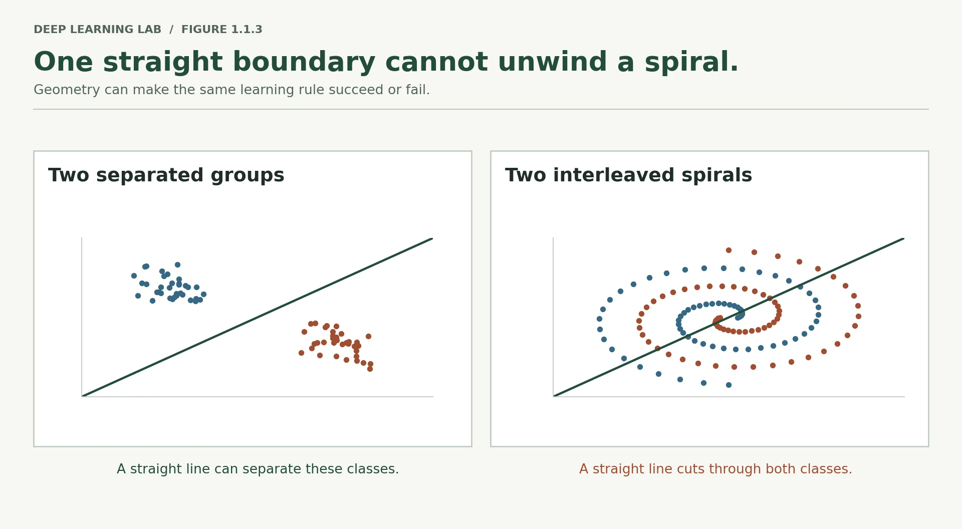
Before you run the next cell, commit to a number. What test accuracy do you expect?
What test accuracy will a logistic regression reach on the raw spirals? (Half the points are in each class, so guessing gives 50%.)
About 60%: the recorded run gives 0.592. Slightly better than a coin flip, because a line can still catch a few more points of one arm on one side of the plane than the other. It cannot follow the arms, so the other ~40% stay wrong however long you train.
Xarray([[-0.55116798, -0.37382426],
[ 0.1575606 , 0.99847351],
[-0.0345203 , 0.07294894],
...,
[-0.98668837, 0.02703767],
[ 0.96692115, -0.14480294],
[ 1.04025859, -0.2036717 ]], shape=(1000, 2))
yarray([0, 0, 0, 1, 0, 1, 1, 0, 1, 1, 1, 0, 0, 1, 0, 1, 1, 0, 0, 1, 0, 1,
0, 0, 0, 1, 0, 0, 0, 1, 1, 0, 0, 0, 1, 1, 1, 1, 0, 0, 0, 0, 1, 0,
1, 1, 0, 1, 1, 0, 1, 1, 1, 1, 0, 0, 1, 1, 1, 0, 0, 0, 0, 0, 0, 0,
0, 1, 0, 1, 1, 0, 0, 1, 0, 0, 0, 0, 1, 1, 0, 1, 0, 0, 1, 0, 0, 0,
1, 0, 0, 0, 0, 0, 1, 1, 1, 0, 0, 0, 1, 0, 1, 1, 1, 1, 1, 1, 0, 1,
1, 0, 1, 0, 0, 0, 1, 1, 1, 1, 1, 1, 1, 0, 1, 0, 1, 0, 1, 1, 0, 0,
1, 0, 0, 0, 1, 0, 1, 0, 0, 0, 0, 0, 0, 1, 0, 0, 0, 1, 1, 0, 0, 1,
1, 1, 0, 0, 1, 0, 1, 0, 0, 1, 0, 1, 0, 0, 1, 1, 0, 0, 0, 1, 0, 1,
0, 0, 0, 1, 0, 0, 0, 1, 1, 1, 1, 1, 0, 1, 1, 1, 0, 1, 0, 0, 0, 0,
1, 1, 1, 0, 1, 1, 1, 0, 1, 1, 0, 0, 0, 0, 1, 1, 0, 1, 0, 1, 1, 0,
0, 1, 1, 1, 0, 0, 0, 1, 0, 0, 1, 0, 1, 1, 0, 0, 0, 0, 0, 1, 0, 0,
1, 0, 1, 1, 1, 0, 1, 1, 0, 1, 1, 1, 0, 0, 1, 0, 1, 0, 1, 1, 1, 1,
1, 0, 1, 0, 1, 1, 0, 0, 0, 0, 0, 1, 1, 1, 1, 0, 0, 1, 0, 1, 0, 0,
1, 1, 1, 1, 0, 0, 1, 0, 0, 1, 1, 0, 0, 1, 0, 0, 0, 1, 1, 0, 0, 0,
1, 0, 1, 0, 1, 0, 0, 0, 1, 0, 1, 0, 1, 1, 0, 0, 0, 0, 0, 0, 1, 1,
1, 0, 0, 1, 1, 0, 0, 0, 1, 1, 1, 0, 0, 1, 1, 0, 1, 1, 1, 1, 0, 1,
1, 1, 1, 1, 0, 0, 1, 1, 1, 0, 0, 1, 0, 1, 1, 0, 0, 0, 1, 1, 1, 1,
0, 1, 1, 1, 0, 0, 1, 1, 1, 0, 0, 1, 0, 1, 1, 1, 1, 0, 0, 1, 1, 1,
1, 0, 1, 1, 1, 0, 0, 1, 0, 0, 0, 0, 1, 1, 1, 0, 0, 1, 0, 0, 1, 0,
1, 1, 1, 0, 1, 1, 1, 1, 0, 1, 1, 1, 1, 0, 0, 1, 1, 0, 0, 0, 1, 0,
0, 0, 0, 0, 1, 1, 0, 0, 1, 1, 1, 1, 1, 0, 1, 0, 1, 0, 1, 0, 1, 1,
1, 1, 1, 1, 1, 0, 1, 0, 1, 1, 0, 1, 1, 1, 1, 0, 1, 1, 1, 1, 0, 0,
1, 0, 1, 0, 1, 1, 0, 0, 1, 1, 0, 0, 0, 1, 0, 1, 1, 0, 0, 0, 1, 0,
0, 0, 0, 0, 1, 1, 1, 1, 0, 0, 0, 0, 0, 0, 1, 0, 0, 0, 0, 0, 0, 0,
1, 1, 1, 0, 1, 0, 0, 0, 0, 1, 0, 1, 1, 1, 0, 1, 1, 1, 1, 0, 1, 0,
1, 1, 0, 1, 1, 1, 1, 0, 0, 0, 1, 1, 0, 0, 0, 0, 1, 1, 0, 1, 1, 0,
1, 0, 0, 0, 0, 1, 0, 1, 0, 1, 1, 1, 1, 0, 1, 0, 0, 1, 1, 1, 0, 1,
0, 1, 0, 0, 0, 1, 1, 1, 0, 0, 0, 0, 1, 1, 1, 0, 1, 1, 0, 1, 1, 1,
1, 0, 0, 0, 0, 0, 0, 1, 0, 0, 1, 0, 0, 0, 0, 0, 1, 0, 1, 1, 0, 0,
0, 0, 1, 0, 1, 0, 0, 1, 1, 0, 1, 0, 0, 1, 0, 1, 0, 1, 0, 0, 0, 0,
1, 0, 0, 0, 1, 1, 0, 1, 1, 0, 1, 0, 0, 0, 1, 0, 1, 0, 1, 1, 1, 1,
0, 0, 0, 1, 1, 1, 1, 1, 0, 0, 0, 1, 1, 0, 0, 1, 1, 0, 0, 1, 1, 1,
1, 0, 1, 0, 1, 0, 1, 0, 0, 0, 0, 1, 0, 1, 0, 0, 0, 1, 1, 1, 0, 0,
0, 0, 0, 0, 1, 1, 1, 0, 1, 0, 0, 0, 1, 1, 1, 0, 1, 1, 1, 1, 1, 1,
1, 1, 0, 1, 0, 0, 0, 0, 1, 0, 1, 1, 0, 1, 1, 1, 0, 1, 0, 0, 1, 0,
1, 1, 0, 1, 1, 0, 1, 1, 0, 1, 1, 0, 1, 0, 1, 0, 1, 1, 1, 0, 0, 0,
0, 1, 0, 1, 0, 0, 0, 0, 0, 0, 0, 1, 0, 0, 0, 0, 0, 0, 1, 1, 1, 1,
0, 1, 0, 1, 1, 0, 1, 0, 1, 0, 0, 0, 1, 0, 1, 1, 1, 1, 1, 1, 1, 1,
0, 0, 0, 1, 1, 1, 1, 0, 1, 0, 1, 0, 0, 1, 0, 0, 0, 0, 1, 0, 1, 1,
1, 1, 0, 0, 1, 1, 1, 0, 1, 1, 1, 0, 1, 0, 0, 1, 1, 0, 0, 1, 1, 1,
1, 1, 1, 0, 0, 0, 0, 0, 0, 0, 1, 0, 1, 0, 1, 1, 1, 1, 0, 1, 1, 1,
0, 1, 1, 1, 0, 0, 0, 1, 1, 1, 0, 1, 0, 0, 0, 1, 1, 0, 1, 1, 0, 0,
0, 1, 0, 0, 1, 0, 0, 0, 0, 0, 0, 0, 0, 1, 1, 1, 1, 0, 1, 1, 1, 1,
0, 0, 0, 0, 0, 1, 0, 0, 1, 0, 1, 0, 1, 1, 1, 1, 0, 1, 0, 0, 0, 1,
1, 1, 0, 1, 1, 1, 0, 1, 1, 1, 0, 1, 0, 0, 1, 1, 0, 0, 0, 0, 0, 1,
1, 0, 1, 0, 1, 0, 0, 0, 1, 1])
from sklearn.model_selection import train_test_splitfrom sklearn.linear_model import LogisticRegressionfrom sklearn.metrics import accuracy_scoreX_train, X_test, y_train, y_test = train_test_split( X, y, test_size=0.25, random_state=0, stratify=y)X_trainarray([[-0.37011545, 0.38877092],
[-0.454673 , -0.20032154],
[ 0.47800824, -0.21109596],
...,
[-0.06792554, 0.27678796],
[ 0.37904385, 0.40279626],
[ 0.38958808, -0.18715052]], shape=(750, 2))
linear = LogisticRegression().fit(X_train, y_train)acc_linear = accuracy_score(y_test, linear.predict(X_test))print(f"Logistic regression on raw (x1, x2): test accuracy = {acc_linear:.3f}")Logistic regression on raw (x1, x2): test accuracy = 0.592
print(f"Always-predict-majority baseline: test accuracy = {max(np.bincount(y_test)) / len(y_test):.3f}")Always-predict-majority baseline: test accuracy = 0.500
def plot_boundary(model, X, y, title, transform=None, ax=None): """Shade a fitted classifier's decision regions and overlay the data. The function lays a fine 300 × 300 grid over the plotting area, asks the model to predict a class for every grid point, and colours each region by its predicted class. The border between the two colours is the model's decision boundary. Args: model: Any fitted scikit-learn classifier with a ``predict`` method. X: Array of shape ``(N, 2)`` with the points to draw. y: Array of shape ``(N,)`` with their true labels (0 or 1). title: Title shown above the plot. transform: Optional function applied to the grid points before predicting. Needed when the model was trained on engineered features (for example ``polar_features``), so it sees inputs in the same form as in training. ax: Matplotlib axes to draw on. A new figure is created when omitted. Returns: The matplotlib axes the plot was drawn on. """ if ax is None: _, ax = plt.subplots(figsize=(5.5, 5.5)) pad = 0.15 x1g = np.linspace(X[:, 0].min() - pad, X[:, 0].max() + pad, 300) x2g = np.linspace(X[:, 1].min() - pad, X[:, 1].max() + pad, 300) G1, G2 = np.meshgrid(x1g, x2g) grid = np.column_stack([G1.ravel(), G2.ravel()]) Z = model.predict(grid if transform is None else transform(grid)).reshape(G1.shape) ax.contourf(G1, G2, Z, alpha=0.25, levels=1, colors=["#3b6ea5", "#d1701c"]) ax.scatter(X[y == 0, 0], X[y == 0, 1], s=6, c="#3b6ea5") ax.scatter(X[y == 1, 0], X[y == 1, 1], s=6, c="#d1701c") ax.set_title(title); ax.set_aspect("equal") ax.set_xlabel("x1"); ax.set_ylabel("x2") return axplot_boundary(linear, X_test, y_test, f"Logistic regression — acc {acc_linear:.3f}")plt.tight_layout(); plt.show()Visualises what a model has learned: it asks the model for a prediction at every point of a fine 300×300 grid covering the plot, shades the grid by the predicted class, and draws the real data on top.
- 1
Creates the grid of (x1, x2) coordinates, 90,000 points in total.
- 2
Predicts a class for every grid point. If the model was trained on engineered features,
transformconverts the grid points first, so the model sees what it saw during training. - 3
Colours the regions, which makes the decision boundary visible.
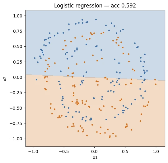
Around 0.59. Barely better than a coin flip, and the picture shows exactly why: one flat blue region, one flat orange region, a single straight seam between them.
Here is the part that matters most, and it is easy to skim past.
Nothing is broken. The data loaded correctly. The labels are perfect. There is no missing data, no leakage, no imbalance. The optimiser converged. There is no bug in the code. The model did precisely what it was designed to do, and the task was simply outside its reach.
That distinction — between a model that failed and a model class that cannot express the answer — is one of the most useful diagnostic instincts you will build in this course. in Module 3 you will need it constantly.
-
If the model is not at fault and the code is not at fault, what exactly is?
The representation, meaning the description of the data the model receives. Logistic regression is handed \((x_1, x_2)\), and in that space the classes are not separable by any straight line. The mismatch is between the model class (straight lines) and the shape of the answer (a coil). Nothing needs debugging; either the description or the model family must change.
-
Would collecting ten times more spiral data improve this result? Why or why not?
No. More data would fill in the spiral arms more densely, but the best straight line through a denser coil is still a straight line through a coil, still about 60%. More data helps a model that is able to express the answer but lacks evidence. It cannot give a model a capability it does not have. (This is sometimes called a problem of bias, not variance.)
-
Would a linear SVM do better? What about a decision tree — and why is the tree a different kind of answer?
- Linear SVM: no better. It also draws one straight line (it just chooses it by a different criterion: the widest margin).
- Decision tree: it can do much better, because it isn't a single line. It chops the plane into many axis-aligned rectangles and can approximate the coil with a staircase of them, given enough depth and data. That is a different kind of answer: the tree gets flexibility by changing the model family, not by learning better features. Its boundary is jagged, needs many splits, and generalises poorly between the arms, which is a hint of why learned smooth features are attractive.
Logistic regression scores about 0.59 on the spirals. Which change would most likely fix it?
More data or more training cannot help: a single straight line cannot trace a coil, whatever the data size. The fix is a different representation or a more expressive model class.
The model 'failed' but nothing is broken. What is the name for this kind of failure?
Distinguishing 'this model failed' from 'this model class cannot represent the answer' is the diagnostic instinct the lesson wants you to build.
Why would ten times more spiral data not rescue logistic regression here?
- Logistic regression draws one straight line in the feature space, by definition.
- The two spiral arms alternate as you move outward, so no straight line separates them in (x1, x2), however many points you have.
- More data only pins down the best straight line more precisely; the limit is the model's expressiveness, not the data.
Fixing it by hand: engineering the features yourself
You are not stuck. You have a whole professional toolkit for exactly this situation, and you have used it many times: if the model cannot express the boundary in the current feature space, change the feature space.
Go back to how you described the rule in Section 2. You almost certainly reached for distance from the centre and angle around the centre. That instinct is correct, and we can write it down.
Each point has a radius \(r = \sqrt{x_1^2 + x_2^2}\) and an angle \(\theta = \arctan2(x_2, x_1)\). Now here is the piece of domain knowledge that unlocks the problem. We built the spirals so that a point's angle grows in lockstep with its radius — that is what makes it a spiral rather than a circle. So if we subtract off the rotation that the radius accounts for, what remains should depend only on which arm the point belongs to.
Define an aligned angle:
For one arm \(\alpha\) lands near \(0\), for the other near \(\pi\). Feed the model \(\sin\alpha\) and \(\cos\alpha\) and the two classes pull apart cleanly. We use sine and cosine rather than \(\alpha\) itself because angles wrap around, and a raw wrapped angle would put nearby points at opposite ends of the number line.
This is unrolling the spiral into a straight strip. Same points, same labels, different description.
def polar_features(Z, revolutions=REVOLUTIONS): """Hand-written features that encode what we know about the spiral's geometry. Keeps the raw coordinates and adds three new columns: the distance from the centre ``r``, and the sine and cosine of the *aligned angle* ``alpha = theta - r * revolutions * 2π``, which removes the twist the radius explains. After this transformation the two arms sit in two separate bands, so a linear model can separate them. It assumes the spiral is centred at (0, 0). Args: Z: Array of shape ``(N, 2)`` with (x1, x2) coordinates. revolutions: Number of turns used when the spirals were generated. The feature only works if this matches the data. Returns: Array of shape ``(N, 5)``: ``[x1, x2, r, sin(alpha), cos(alpha)]``. """ r = np.sqrt(Z[:, 0] ** 2 + Z[:, 1] ** 2) theta = np.arctan2(Z[:, 1], Z[:, 0]) alpha = theta - r * (revolutions * 2 * np.pi) # remove the rotation the radius explains return np.column_stack([Z, r, np.sin(alpha), np.cos(alpha)])Your hand-written representation: keeps x1 and x2 and adds three new columns that encode the spiral geometry.
- 1
Distance from the centre, \(\sqrt{x_1^2 + x_2^2}\). It assumes the centre is (0, 0)!
- 2
Direction from the centre, in radians (−π to π).
- 3
Removes the twist that the radius explains, leaving roughly 0 for one arm and π for the other.
- 4
Five columns go to the linear model: x1, x2, r, sin α, cos α.
X_trainarray([[-0.37011545, 0.38877092],
[-0.454673 , -0.20032154],
[ 0.47800824, -0.21109596],
...,
[-0.06792554, 0.27678796],
[ 0.37904385, 0.40279626],
[ 0.38958808, -0.18715052]], shape=(750, 2))
polar_features(X_train)array([[-0.37011545, 0.38877092, 0.53677581, 0.18212516, 0.98327536],
[-0.454673 , -0.20032154, 0.49684631, 0.89403051, -0.44800608],
[ 0.47800824, -0.21109596, 0.5225451 , -0.71791249, -0.69613336],
...,
[-0.06792554, 0.27678796, 0.2850008 , -0.45845638, -0.88871691],
[ 0.37904385, 0.40279626, 0.55309951, -0.99983226, -0.01831514],
[ 0.38958808, -0.18715052, 0.4322085 , -0.81559639, 0.57862123]],
shape=(750, 5))
linear_fe = LogisticRegression(max_iter=3000).fit(polar_features(X_train), y_train)acc_fe = accuracy_score(y_test, linear_fe.predict(polar_features(X_test)))print(f"Logistic regression, engineered features: {acc_fe:.3f}")Logistic regression, engineered features: 0.992
print(f"Logistic regression, raw features: {acc_linear:.3f}")Logistic regression, raw features: 0.592
plot_boundary(linear_fe, X_test, y_test, f"Same linear model, better features — acc {acc_fe:.3f}", transform=polar_features)plt.tight_layout(); plt.show()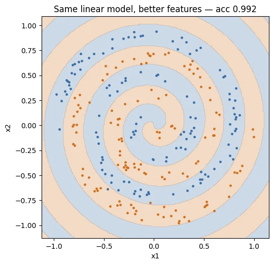
From 0.59 to 0.99. The model never changed — it is the same logistic regression, still drawing a single straight line. What changed is the space it draws that line in. In the aligned-angle space, one straight cut is all the problem ever needed.
This is worth stating plainly because it is the hinge of the whole argument:
The limitation was never in the classifier. It was in the representation.
Same model, different space
Logistic regression → 0.592. The line has to cut through a coil.
The same logistic regression → 0.992. In this space the classes sit in two clean bands.
-
The engineered version beats the network we are about to train. Is engineering features therefore the better technique here?
Here, yes. In general, no. The engineered version wins (0.99 vs 0.95) and is cheaper, faster and fully interpretable. But it only exists because you knew the generating process. The better technique depends on the situation: when you have that knowledge and the structure is simple, write the feature. When you don't (images, audio, text), you can't. The honest comparison is not "features vs networks" but "your knowledge vs the model's data".
-
How much did you need to know about how the data was generated to invent
alpha? Could you have derived it from the scatter plot alone?A lot: that the data is a spiral, where its centre is, and exactly how many revolutions it makes (the
revolutionsvalue is baked into the formula for \(\alpha\)). From the scatter plot alone you could guess radius and angle matter and maybe estimate the number of turns by counting, but getting the exact "twist" parameter right would take trial and error. In real problems you usually don't have the generating equations at all. -
What happens to
polar_featuresif the spirals are not centred at the origin?They quietly break.
polar_featuresmeasures radius and angle from (0, 0). If the spiral is centred elsewhere, \(r\) and \(\theta\) no longer describe position along the arm, \(\alpha\) no longer lines up the arms, and the linear model's accuracy collapses, with no error message. You can see this in the Spiral Lab by moving the centre. The network, by contrast, simply re-learns from the new coordinates. Hand-made features encode your assumptions, and when the assumptions stop being true, the features fail silently.
Write the hand-made features yourself
Complete aligned_features so it returns the radius \(r\), \(\sin\alpha\) and \(\cos\alpha\) for each point, exactly as §4 defines
them. Replace every ___, then press Check my code.
After adding r, sin α and cos α, the same logistic regression jumps from 0.59 to 0.99. What changed?
The classifier is unchanged and still draws one straight line. In the aligned-angle space one straight cut is all the problem needs. The limitation was in the representation.
Why feed the model sin α and cos α rather than α itself?
An angle of 359° is next to 1°, but as a raw number they are far apart. sin and cos place wrapped angles smoothly next to each other.
In two sentences: what did you have to know to invent the aligned angle α, and why does that matter?
- You needed to know how the data was generated: the angle grows in lockstep with the radius (the number of revolutions).
- That knowledge rarely comes with real data, so hand-engineering like this only works when you can see and understand the structure.
Who invented those features?
You did.
And that is fine — for this problem. You could see the data in two dimensions, you knew the generating process, and the geometry was simple enough to reason about over a coffee. Under those conditions, hand-engineering is not merely acceptable, it is often the superior engineering decision: it is fast, cheap, interpretable, and it encodes real knowledge that no amount of data can supply.
So ask the uncomfortable question. What are the actual preconditions for what you just did?
- You could visualise the data. Two dimensions. Now imagine 4,096.
- You knew the generating process. You wrote it. Real data rarely comes with its equations attached.
- The right transformation was compact — one line of trigonometry. Not every structure compresses that well.
- The features were stable. Change the centre, the number of revolutions, or the noise level and
polar_featuresdegrades.
Strip away any one of those and the approach starts to strain. Strip away all four — which is the normal condition for images, audio, and text — and it collapses entirely. Section 10 shows you exactly what that collapse looks like.
This is the gap deep learning was built to fill. Not "features are bad." Rather: when you cannot invent the features, you need a method that discovers them from the data, as part of solving the task.
-
Think about a domain you know well. Roughly how long would it take a newcomer to learn the features that experts in that domain consider obvious? That duration is a rough estimate of what representation learning is trying to compress.
There is no single right number; the point is the order of magnitude. A radiologist learns to read chest X-rays over years of training; a fraud analyst learns the telltale transaction patterns over months; a sommelier trains for years. Representation learning tries to compress that apprenticeship into training time on data. That is why it needs so many examples: it is learning, from scratch, what an expert learned from thousands of cases and a mentor.
Which condition, when missing, makes hand-engineering features like α collapse for images, audio and text?
Hand-engineering relied on seeing the data in 2-D, knowing how it was made, a compact transformation and stable structure. Pixels, waveforms and text usually lack all four.
A small network finds them on its own
Now we hand a neural network the raw x1 and x2 columns. No radius. No angle. No trigonometry. Nothing of what you worked out in Section 4.
We use scikit-learn's MLPClassifier here deliberately, because the point of this section is the result, not the mechanism. Lesson 1.2 opens up the mechanism by hand, and Lesson 1.3 rebuilds it in PyTorch. For now, treat it as a black box that we are about to justify opening.
from sklearn.neural_network import MLPClassifierimport timet0 = time.time()net = MLPClassifier( hidden_layer_sizes=(64, 64), # two hidden layers, 64 units each activation="relu", learning_rate_init=0.01, max_iter=6000, random_state=0,).fit(X_train, y_train) # <-- raw x1, x2 onlytrain_time = time.time() - t0A small neural network from scikit-learn. It gets only the raw X_train (x1, x2), with no engineered features.
- 1
Two hidden layers of 64 units each. These layers will learn the features.
- 2
ReLU, \(\max(0, z)\), is the non-linearity that lets the network bend its boundary. Lesson 1.2 shows why it is essential.
- 3
Step size for the optimiser (Adam). Module 3 is about choosing it.
- 4
Upper limit on training passes (epochs) over the data.
acc_net = accuracy_score(y_test, net.predict(X_test))acc_net0.952
n_params = sum(w.size for w in net.coefs_) + sum(b.size for b in net.intercepts_)print(f"Linear, raw features: {acc_linear:.3f}")print(f"Linear, engineered features: {acc_fe:.3f} <- required your domain knowledge")print(f"Neural network, raw features:{acc_net:.3f} <- required none")print(f"\nNetwork parameters: {n_params:,} | training time: {train_time:.1f}s")Linear, raw features: 0.592 Linear, engineered features: 0.992 <- required your domain knowledge Neural network, raw features:0.952 <- required none Network parameters: 4,417 | training time: 0.2s
plot_boundary(net, X_test, y_test, f"Neural network on raw features — acc {acc_net:.3f}")plt.tight_layout(); plt.show()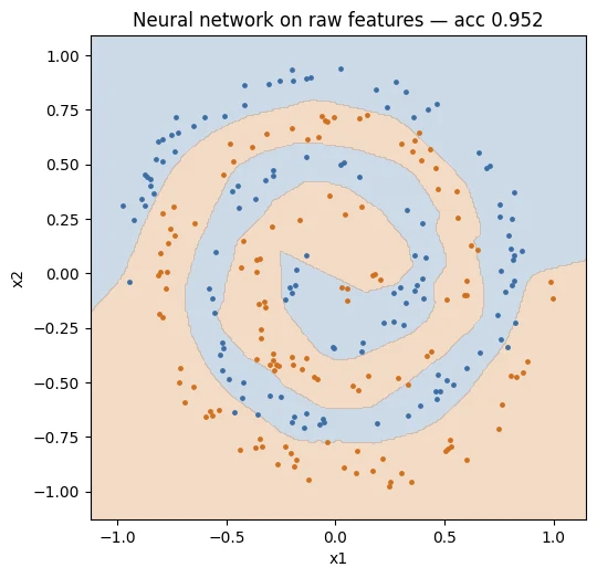
The boundary curves. It wraps around the arms, follows the spiral outward, and does so without anyone telling it that spirals have a radius and an angle.
Something specific happened inside that model, and naming it correctly matters more than being impressed by it. The network's first layer transformed (x1, x2) into 64 new numbers. The second layer transformed those into 64 more. Only the final layer performed the classification — and it is, in essence, a logistic regression, exactly like the one that failed in Section 3.
So the last layer is the same model that could not solve this problem. What changed is that it now sits on top of a representation the network built for itself. The earlier layers are the feature engineering. They were fitted, not written.
Ringed dots are test points the model never trains on; the accuracy shown is measured on them. Numbers differ a little from the notebook (different random seed and optimiser settings), but the pattern is the same: linear ≈ 60%, engineered ≈ 99%, network ≈ 95%+.
Train the neural network to at least 95% test accuracy with at most 300 parameters. Fewer is better: change Hidden units per layer and Hidden layers, then train.
-
The network reached 0.95 while your engineered features reached 0.99. Which approach would you defend in a design review, and what would decide it?
It depends on what the design review cares about, and a good answer names the deciding factors:
- Stability of the data: if the generating process could shift (new centre, different spirals), the network is more robust; the hand-made features fail silently.
- Interpretability and cost: the engineered model is tiny, fast and explainable. If those matter most and the process is fixed, defend it.
- Maintenance: who will update
polar_featureswhen the data changes? A learned representation updates by retraining.
A strong answer: "Ship the engineered model if the data-generating process is known and stable. Otherwise ship the network, and monitor it."
-
The network used roughly 4,000 parameters to learn what you expressed in three. What did it buy with that extra capacity?
Flexibility. Your three features are correct for this exact spiral. The network's ~4,400 parameters can represent a huge family of curved boundaries, so it could just as well fit a spiral with a different centre, a different number of turns, or a completely different shape, without anyone rewriting code. The price is that it needs more data to pin those parameters down, and it can overfit when data is scarce.
-
What would happen if you trained this same network on 50 points instead of 1,000? Try it — change
n_per_classand re-run. The result is the seed of a lesson we return to in Module 7.With only 50 points, the network has far more parameters (~4,400) than examples, so it can memorise the training points: training accuracy near 100%, test accuracy much lower, with a wiggly boundary that fits noise rather than the spiral. That gap between train and test performance is overfitting, and it is why pretrained models (Module 7) matter: they bring a representation learned on huge data, so you need fewer examples of your own. Try it in the Spiral Lab by setting Points per class to 25.
The network's final layer is essentially the same logistic regression that failed in §3. Why does it now succeed?
The earlier layers are the feature engineering, fitted rather than written. The final straight cut works because it is made in the learned space.
Explain what the hidden layers of the network are doing, using the phrase 'fitted, not written'.
- The hidden layers transform (x1, x2) into new numbers, a learned description of each point, just as r and α were a hand-written one.
- Those transformations are learned by training (fitted), not designed by a person (written); the last layer then classifies in that learned space.
The honest counterexample: churn, where the network wins nothing
If this lesson stopped at Section 6, you would leave with a conclusion that is both tidy and wrong: neural networks learn their own features, therefore neural networks are better.
They are not better. They are different, and the difference pays off only under specific conditions. The fastest way to see this is to run the comparison on the kind of data most working data scientists actually face.
We use the Telco Customer Churn dataset — 7,043 customers, 20 predictors, a binary churn label. It is tabular, mixed categorical and numeric, moderately imbalanced. If you have worked in industry, you have met a dozen datasets shaped exactly like this.
Both models get the same split, the same preprocessing, and a fair shot.
URLS = [ "https://raw.githubusercontent.com/IBM/telco-customer-churn-on-icp4d/master/data/Telco-Customer-Churn.csv", "https://raw.githubusercontent.com/treselle-systems/customer_churn_analysis/master/WA_Fn-UseC_-Telco-Customer-Churn.csv",]churn = Nonefor url in URLS: try: churn = pd.read_csv(url) print(f"Loaded from: {url.split('/')[4]}") break except Exception as e: print(f" failed ({type(e).__name__}), trying next mirror...")if churn is None: raise RuntimeError("Could not download the dataset. Check your internet connection.")print("shape:", churn.shape)churn.head(3)Downloads the Telco churn CSV, trying a second mirror if the first fails, and stops with a clear error if neither works.
Loaded from: telco-customer-churn-on-icp4d
shape: (7043, 21)
| customerID | gender | SeniorCitizen | Partner | Dependents | tenure | PhoneService | MultipleLines | InternetService | OnlineSecurity | ... | DeviceProtection | TechSupport | StreamingTV | StreamingMovies | Contract | PaperlessBilling | PaymentMethod | MonthlyCharges | TotalCharges | Churn | |
|---|---|---|---|---|---|---|---|---|---|---|---|---|---|---|---|---|---|---|---|---|---|
| 0 | 7590-VHVEG | Female | 0 | Yes | No | 1 | No | No phone service | DSL | No | ... | No | No | No | No | Month-to-month | Yes | Electronic check | 29.85 | 29.85 | No |
| 1 | 5575-GNVDE | Male | 0 | No | No | 34 | Yes | No | DSL | Yes | ... | Yes | No | No | No | One year | No | Mailed check | 56.95 | 1889.5 | No |
| 2 | 3668-QPYBK | Male | 0 | No | No | 2 | Yes | No | DSL | Yes | ... | No | No | No | No | Month-to-month | Yes | Mailed check | 53.85 | 108.15 | Yes |
churn.info()<class 'pandas.core.frame.DataFrame'> RangeIndex: 7043 entries, 0 to 7042 Data columns (total 21 columns): # Column Non-Null Count Dtype --- ------ -------------- ----- 0 customerID 7043 non-null object 1 gender 7043 non-null object 2 SeniorCitizen 7043 non-null int64 3 Partner 7043 non-null object 4 Dependents 7043 non-null object 5 tenure 7043 non-null int64 6 PhoneService 7043 non-null object 7 MultipleLines 7043 non-null object 8 InternetService 7043 non-null object 9 OnlineSecurity 7043 non-null object 10 OnlineBackup 7043 non-null object 11 DeviceProtection 7043 non-null object 12 TechSupport 7043 non-null object 13 StreamingTV 7043 non-null object 14 StreamingMovies 7043 non-null object 15 Contract 7043 non-null object 16 PaperlessBilling 7043 non-null object 17 PaymentMethod 7043 non-null object 18 MonthlyCharges 7043 non-null float64 19 TotalCharges 7043 non-null object 20 Churn 7043 non-null object dtypes: float64(1), int64(2), object(18) memory usage: 1.1+ MB
# TotalCharges arrives as text with blanks for brand-new customerschurn["TotalCharges"] = pd.to_numeric(churn["TotalCharges"], errors="coerce").fillna(0.0)y_churn = (churn["Churn"] == "Yes").astype(int).valuesX_churn = pd.get_dummies(churn.drop(columns=["customerID", "Churn"]), drop_first=True).astype(float)print("features after one-hot encoding:", X_churn.shape[1])print("churn rate:", f"{y_churn.mean():.1%}")Turns the raw table into numbers a model can use.
- 1
TotalChargesarrives as text; brand-new customers have a blank.errors="coerce"turns blanks into NaN, thenfillna(0.0)sets them to 0. - 2
The label: 1 if the customer churned (
"Yes"), else 0. - 3
One-hot encoding: every categorical column becomes several 0/1 columns, one per category.
drop_first=Truedrops one redundant column per category. The ID column is dropped because it carries no signal.
features after one-hot encoding: 30
churn rate: 26.5%
X_churn| SeniorCitizen | tenure | MonthlyCharges | TotalCharges | gender_Male | Partner_Yes | Dependents_Yes | PhoneService_Yes | MultipleLines_No phone service | MultipleLines_Yes | ... | StreamingTV_No internet service | StreamingTV_Yes | StreamingMovies_No internet service | StreamingMovies_Yes | Contract_One year | Contract_Two year | PaperlessBilling_Yes | PaymentMethod_Credit card (automatic) | PaymentMethod_Electronic check | PaymentMethod_Mailed check | |
|---|---|---|---|---|---|---|---|---|---|---|---|---|---|---|---|---|---|---|---|---|---|
| 0 | 0.0 | 1.0 | 29.85 | 29.85 | 0.0 | 1.0 | 0.0 | 0.0 | 1.0 | 0.0 | ... | 0.0 | 0.0 | 0.0 | 0.0 | 0.0 | 0.0 | 1.0 | 0.0 | 1.0 | 0.0 |
| 1 | 0.0 | 34.0 | 56.95 | 1889.50 | 1.0 | 0.0 | 0.0 | 1.0 | 0.0 | 0.0 | ... | 0.0 | 0.0 | 0.0 | 0.0 | 1.0 | 0.0 | 0.0 | 0.0 | 0.0 | 1.0 |
| 2 | 0.0 | 2.0 | 53.85 | 108.15 | 1.0 | 0.0 | 0.0 | 1.0 | 0.0 | 0.0 | ... | 0.0 | 0.0 | 0.0 | 0.0 | 0.0 | 0.0 | 1.0 | 0.0 | 0.0 | 1.0 |
| 3 | 0.0 | 45.0 | 42.30 | 1840.75 | 1.0 | 0.0 | 0.0 | 0.0 | 1.0 | 0.0 | ... | 0.0 | 0.0 | 0.0 | 0.0 | 1.0 | 0.0 | 0.0 | 0.0 | 0.0 | 0.0 |
| 4 | 0.0 | 2.0 | 70.70 | 151.65 | 0.0 | 0.0 | 0.0 | 1.0 | 0.0 | 0.0 | ... | 0.0 | 0.0 | 0.0 | 0.0 | 0.0 | 0.0 | 1.0 | 0.0 | 1.0 | 0.0 |
| ... | ... | ... | ... | ... | ... | ... | ... | ... | ... | ... | ... | ... | ... | ... | ... | ... | ... | ... | ... | ... | ... |
| 7038 | 0.0 | 24.0 | 84.80 | 1990.50 | 1.0 | 1.0 | 1.0 | 1.0 | 0.0 | 1.0 | ... | 0.0 | 1.0 | 0.0 | 1.0 | 1.0 | 0.0 | 1.0 | 0.0 | 0.0 | 1.0 |
| 7039 | 0.0 | 72.0 | 103.20 | 7362.90 | 0.0 | 1.0 | 1.0 | 1.0 | 0.0 | 1.0 | ... | 0.0 | 1.0 | 0.0 | 1.0 | 1.0 | 0.0 | 1.0 | 1.0 | 0.0 | 0.0 |
| 7040 | 0.0 | 11.0 | 29.60 | 346.45 | 0.0 | 1.0 | 1.0 | 0.0 | 1.0 | 0.0 | ... | 0.0 | 0.0 | 0.0 | 0.0 | 0.0 | 0.0 | 1.0 | 0.0 | 1.0 | 0.0 |
| 7041 | 1.0 | 4.0 | 74.40 | 306.60 | 1.0 | 1.0 | 0.0 | 1.0 | 0.0 | 1.0 | ... | 0.0 | 0.0 | 0.0 | 0.0 | 0.0 | 0.0 | 1.0 | 0.0 | 0.0 | 1.0 |
| 7042 | 0.0 | 66.0 | 105.65 | 6844.50 | 1.0 | 0.0 | 0.0 | 1.0 | 0.0 | 0.0 | ... | 0.0 | 1.0 | 0.0 | 1.0 | 0.0 | 1.0 | 1.0 | 0.0 | 0.0 | 0.0 |
Xc_train, Xc_test, yc_train, yc_test = train_test_split( X_churn.values, y_churn, test_size=0.25, random_state=0, stratify=y_churn)from sklearn.ensemble import HistGradientBoostingClassifierfrom sklearn.preprocessing import StandardScalerfrom sklearn.metrics import roc_auc_score# Gradient boosting: no scaling needed, handles mixed feature scales nativelyt0 = time.time()gbdt = HistGradientBoostingClassifier(random_state=0).fit(Xc_train, yc_train)gbdt_time = time.time() - t0gbdt_auc = roc_auc_score(yc_test, gbdt.predict_proba(Xc_test)[:, 1])Trains gradient-boosted trees and scores them by ROC-AUC on the test set.
- 1
Gradient boosting builds many small decision trees, each correcting the errors of the previous ones. The Hist version bins features first, which makes it fast. It uses default settings, with no tuning.
- 2
Probability of class 1 (churn) for every test customer; AUC is computed from these scores.
gbdt_auc0.829237396119133
# Neural network: scaling is NOT optional here — we will return to why in Module 3scaler = StandardScaler().fit(Xc_train)t0 = time.time()mlp = MLPClassifier(hidden_layer_sizes=(64, 32), max_iter=500, random_state=0)mlp.fit(scaler.transform(Xc_train), yc_train)mlp_time = time.time() - t0mlp_auc = roc_auc_score(yc_test, mlp.predict_proba(scaler.transform(Xc_test))[:, 1])The network needs standardised inputs. The scaler learns each column's mean and standard deviation from the training set only, then applies them to both sets.
- 1
Fit on train only. Fitting on the test set would leak information about it (Module 4, Lesson 4.1).
- 2
Two hidden layers, 64 then 32 units.
mlp_auc0.7738739827038977
print(f"{'model':<22}{'ROC-AUC':>10}{'train time':>14}")print("-" * 46)print(f"{'Gradient boosting':<22}{gbdt_auc:>10.4f}{gbdt_time:>13.1f}s")print(f"{'Neural network':<22}{mlp_auc:>10.4f}{mlp_time:>13.1f}s")model ROC-AUC train time ---------------------------------------------- Gradient boosting 0.8292 2.8s Neural network 0.7739 2.0s
Gradient boosting wins on quality and costs roughly a tenth of the training time. It also needed no feature scaling, exposes feature importances for free, and has far fewer knobs to get wrong.
This is not a fluke of one dataset or one seed. On medium-sized tabular data with meaningful engineered columns, gradient-boosted trees remain a genuinely strong default in 2026 — a fact that survives every wave of deep learning enthusiasm, and one that experienced practitioners take for granted.
Why? The spiral had geometric structure in raw coordinates that a network could exploit. The churn table does not. Its columns are already meaningful, human-curated quantities — tenure, monthly charge, contract type. Someone already did the representation learning, by hand, when they designed the database schema. There is very little left for a network to discover.
That gives you a usable heuristic, and it is worth committing to memory:
Deep learning pays off where the raw signal is high-dimensional, redundant, and structured in ways humans cannot easily write down — pixels, waveforms, text. On well-curated tabular data, it frequently does not.
-
Your manager asks for a churn model by Friday. Which do you build, and what would change your answer?
Build gradient boosting. On curated tabular data it is usually as accurate or more accurate, trains quickly, needs no feature scaling, has few hyperparameters, and gives feature importances you can show your manager on Friday.
What would change the answer: very large data (millions of rows), raw unstructured inputs attached to each customer (call transcripts, clickstreams, images), a need to share one learned representation across many tasks, or a proper bake-off (Module 4) in which the network actually wins.
-
Under what circumstances would you expect a network to beat gradient boosting on tabular data?
When the table isn't really "curated tabular data":
- columns hold raw, high-dimensional signals (text fields, sequences of events, embedded images);
- there are very high-cardinality categories (millions of user IDs) where learned embeddings shine;
- the dataset is huge and the relationships are subtle;
- you want to combine tabular data with other modalities in one model, or transfer knowledge from a pretrained model.
-
We tuned neither model. Does that weaken the conclusion? What would a fair comparison require? Hold that thought — it is the whole of Module 4.
It weakens it a little, but not much. Tuning can move each model by a few points, so a fair comparison needs: the same splits (ideally several random splits or cross-validation), equal tuning budgets for both models, the same preprocessing information, a report of variance across runs rather than one number, and a check of cost (time, memory, complexity). Industry experience and published benchmarks agree with the direction of this result: on medium-sized tabular data, tuned gradient boosting is usually at least as strong. Module 4's bake-off does it properly.
On the Telco churn table, gradient boosting beat the network (0.829 vs 0.774 AUC). What is the lesson's explanation?
Someone already did the representation learning when designing the schema (tenure, charges, contract type). Networks pay off where the raw signal is high-dimensional and unstructured.
State the lesson's rule of thumb for when deep learning pays off, and when it usually does not.
- Deep learning pays off when the raw signal is high-dimensional, redundant and structured in ways people cannot write down: pixels, waveforms, text.
- On well-curated tabular data with meaningful columns, gradient-boosted trees are usually a strong (often better, cheaper) default.
What actually changed
Three experiments, three results. Let us extract the principle carefully, because loose versions of it are everywhere and most of them are wrong.
| Feature engineering | Model | Result | |
|---|---|---|---|
| Spirals, linear | You wrote r, sin α, cos α |
Logistic regression | 0.99 |
| Spirals, network | None | 2-layer network | 0.95 |
| Churn, boosting | Schema designers, years ago | Gradient boosting | 0.829 AUC |
| Churn, network | Same schema | 2-layer network | 0.774 AUC |
Here is the principle:
Representation learning means the transformation from raw input to useful description is learned from data, jointly with the task, rather than specified in advance by a person.
Three things this does not say, each corresponding to a claim you will encounter and should push back on:
- It does not say feature engineering is obsolete. Section 4 outperformed Section 6.
- It does not say networks always win. Section 7 says the opposite, on the data type most companies hold most of.
- It does not say the work vanishes. It moves — into architecture choice, data preparation, and training dynamics. Modules 2 through 4 are about that relocated work.
What it does say is that a door opened. Once representations are learnable, you can attack problems where nobody knows how to write the features down — and you can reuse a representation learned on one task for a different task. That second consequence is transfer learning, it is the basis of every pretrained model you will touch from Module 7 onward, and it is why this idea matters far beyond the accuracy numbers above.
-
Rewrite the principle above in your own words, in two sentences, without using the words "features" or "representation". If you cannot, reread the table.
Example: "In older methods, a person decides how to describe each example and the algorithm only learns the final decision. In deep learning, the system learns how to describe the examples at the same time as it learns the decision, from the same data."
If your version says who does the describing and when it is learned, you have the principle.
Which statement follows from 'representation learning' as the lesson defines it?
The principle says the description can be learned from data jointly with the task. It does not say networks always win or that engineering vanishes; the work moves.
Rewrite the lesson's principle in two sentences without using the words 'features' or 'representation'.
- The step that turns raw input into a useful description is learned from examples, at the same time as the task, instead of being designed by a person.
- This matters most where people cannot write that step down, and it lets a description learned on one task be reused on another (transfer learning).
Where feature engineering still lives in deep learning
A tempting summary of Section 6 is that the network needed no preparation. That is false, and believing it will cost you real time in Module 3.
Watch what happens when we remove one preprocessing step from the churn network — the standardisation that we quietly applied.
mlp_unscaled = MLPClassifier(hidden_layer_sizes=(64, 32), max_iter=500, random_state=0)mlp_unscaled.fit(Xc_train, yc_train) # same model, same data, NO scalingauc_unscaled = roc_auc_score(yc_test, mlp_unscaled.predict_proba(Xc_test)[:, 1])print(f"Neural network, standardised inputs: {mlp_auc:.4f}")print(f"Neural network, raw inputs: {auc_unscaled:.4f}")print(f"\nDamage from skipping one preprocessing step: {mlp_auc - auc_unscaled:.4f} AUC")print(f"\nFeature ranges in the raw data:")print(f" tenure: {Xc_train[:, X_churn.columns.get_loc('tenure')].min():.1f} to " f"{Xc_train[:, X_churn.columns.get_loc('tenure')].max():.1f}")print(f" TotalCharges: {Xc_train[:, X_churn.columns.get_loc('TotalCharges')].min():.1f} to " f"{Xc_train[:, X_churn.columns.get_loc('TotalCharges')].max():.1f}")Neural network, standardised inputs: 0.7739 Neural network, raw inputs: 0.7794 Damage from skipping one preprocessing step: -0.0056 AUC Feature ranges in the raw data: tenure: 0.0 to 72.0 TotalCharges: 0.0 to 8672.5
One column spans single digits, another spans thousands. Gradient descent takes steps that are the same size in every direction, so a feature measured in thousands dominates the update and a feature measured in tens is effectively ignored for a long time. Module 3 makes this precise. For now, note the empirical fact: the "no feature engineering needed" model lost real performance from a missing three-line transformation.
So where does the human work actually live in a deep learning project in 2026?
- Input scaling and normalisation — never optional, as you just measured.
- Data quality and labelling — the single largest lever on final performance, and Module 8 is devoted to it.
- Architecture choice — a convolution encodes "nearby pixels are related"; attention encodes "any token may relate to any other". These are engineered inductive biases, chosen by you.
- Tokenisation for text, sample rate for audio, image resizing and augmentation for vision — all human decisions made before the model sees anything.
- Loss design — what you optimise defines what you get.
The work did not disappear. It changed shape, and it moved up a level of abstraction.
Try a large learning rate (above 1.0) with raw features to see the zig-zag, and above 2.0 to see it diverge. Then press Standardised: the valley becomes a round bowl and the same algorithm arrives in a handful of steps.
Where the human work lives in a deep learning project
Put features on comparable scales before training.
Often the biggest lever on final performance (Module 8).
Built-in assumptions, e.g. nearby pixels are related (convolution).
Text tokens, audio sample rate, image size and augmentation.
What you optimise is what you get.
-
Of the five items above, which do you think is most often responsible for a deep learning project underperforming in production? Write your answer down and revisit it in Module 8.
Most practitioners would say data quality and labelling. In production, models usually fail because the data they see differs from the training data (distribution shift), labels were noisy or inconsistent, or important cases were missing, not because the architecture was wrong. Architecture and loss design matter, but a mediocre architecture on excellent data usually beats an excellent architecture on poor data. Module 4 (data you can trust) and Module 8 (data engineering) are built around this. Keep your written answer and compare it when you get there.
Why can unscaled inputs hurt a network trained with gradient descent?
Gradient descent's steps interact with each feature's scale. TotalCharges (0–8,672) swamps tenure (0–72) unless inputs are standardised. Module 3 makes this precise.
Name two places where human engineering effort still lives in a deep learning project, and say why each matters.
- Any two of: input scaling/normalisation; data quality and labelling; architecture choice (an engineered inductive bias); tokenisation / sample rate / resizing and augmentation; loss design.
- Each shapes what the network can learn before or while it trains, so the work moved rather than disappeared.
Raw pixels: the point of no return
The spirals had two features. You could plot them, reason about them, and invent a transformation over lunch. Now we scale the input up, and the argument stops being a matter of taste.
These are 8×8 handwritten digits — 64 pixels each, the smallest realistic image data that exists. Modern images are hundreds of times larger.
from sklearn.datasets import load_digitsdigits = load_digits()print("images:", digits.images.shape, " -> flattened:", digits.data.shape)print("classes:", np.unique(digits.target))images: (1797, 8, 8) -> flattened: (1797, 64) classes: [0 1 2 3 4 5 6 7 8 9]
fig, axes = plt.subplots(2, 8, figsize=(11, 3))for ax, img, label in zip(axes.ravel(), digits.images, digits.target): ax.imshow(img, cmap="gray_r"); ax.set_title(str(label), fontsize=9); ax.axis("off")plt.suptitle("Each of these is 64 numbers between 0 and 16", y=1.02)plt.tight_layout(); plt.show()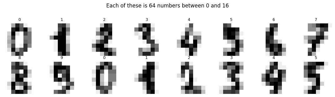
Now try to do what you did in Section 4. Write a feature that separates 3 from 8.
Not a model — a feature. An explicit arithmetic function of those 64 pixel values that is reliably larger for one digit than the other. Give yourself two honest minutes before running the next cell.
# The kind of feature a person actually reaches for first: overall darkness.ink = digits.data.mean(axis=1)mask = np.isin(digits.target, [3, 8])ink_38, lab_38 = ink[mask], digits.target[mask]fig, ax = plt.subplots(figsize=(7, 3.2))ax.hist(ink_38[lab_38 == 3], bins=30, alpha=0.6, label="digit 3", color="#3b6ea5")ax.hist(ink_38[lab_38 == 8], bins=30, alpha=0.6, label="digit 8", color="#d1701c")ax.set_xlabel("mean pixel intensity ('how much ink')"); ax.set_ylabel("count")ax.set_title("A hand-designed feature, meeting reality"); ax.legend()plt.tight_layout(); plt.show()# How far does that one feature get us?thresh = ink_38.mean()pred = np.where(ink_38 > thresh, 8, 3)print(f"Accuracy from 'total ink' alone, 3 vs 8: {(pred == lab_38).mean():.3f}")Tries the most natural hand-made feature, total ink, to separate 3 from 8, then measures how well a simple threshold on it works.
- 1
One number per image: the average of its 64 pixel values.
- 2
A simple rule: call it an 8 if it has more ink than average, otherwise a 3.
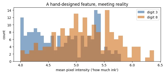
Accuracy from 'total ink' alone, 3 vs 8: 0.625
The distributions sit almost on top of each other. And this was the easy pair, on 8×8 images, distinguishing only two classes.
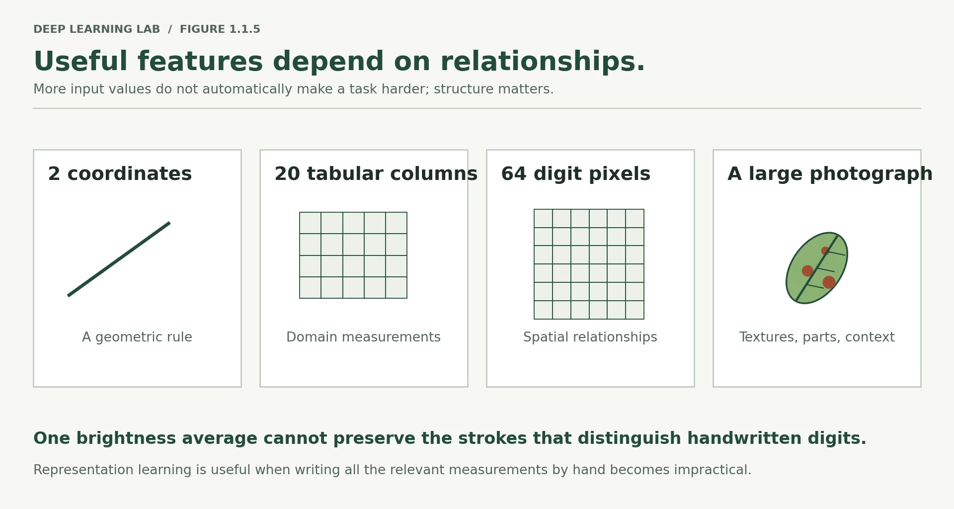
Now consider what you are actually up against. Distinguishing all ten digits needs features robust to stroke thickness, slant, position, size and writing style. A 224×224 colour photograph has 150,528 numbers. The pixel at position 9,412 means nothing on its own — meaning lives in relationships between pixels, across many scales at once, and those relationships shift when the object moves two pixels to the left.
No one hand-writes that. People genuinely tried, for decades, with real ingenuity — SIFT, HOG, wavelet banks, Gabor filters. Those were serious engineering achievements, and learned representations comprehensively outperformed them.
Deep diveWhat were SIFT, HOG and Gabor filters?
Before about 2012, computer vision ran on hand-designed feature extractors:
- Gabor filters / wavelets: fixed patterns that respond to edges and textures at particular orientations and scales.
- SIFT (Scale-Invariant Feature Transform): finds distinctive keypoints and describes the gradient directions around them, built to survive scaling and rotation.
- HOG (Histogram of Oriented Gradients): counts edge directions in small cells. It was famous for pedestrian detection.
These were brilliant pieces of engineering. In 2012 a convolutional network (AlexNet) trained on ImageNet beat them by a wide margin, and its first-layer filters turned out to look strikingly like Gabor filters. The network learned the features people had spent decades designing, and then went further.
-
Why does the pixel at a fixed position carry so little information on its own?
Because meaning comes from patterns, not positions. Pixel (3, 4) is dark in a 7, a 2 and a shifted 1. The same digit written slightly to the left, thicker, or slanted lights up completely different positions. Any single pixel is only weakly and unreliably related to the label. The information is in the relationships between pixels (strokes, loops, corners), which no single number captures. Try it in the Pixel Lab: a one-pixel shift changes many of the 64 numbers.
-
Digit images are centred and size-normalised. What breaks if they are not?
Everything that depends on fixed positions. If digits can appear anywhere in the frame at any size, a pixel-position feature (or a simple model that treats each pixel as a fixed column) sees an almost unrelated input for the same digit. You would need features that are invariant to translation and scale, which is exactly what hand-engineered vision systems (SIFT, HOG) spent decades trying to build, and what convolutional networks build in by design (Module 5 discusses CNNs).
-
Given the difficulty above, why does a network learning these features from scratch not seem hopeless? What does it have that you do not?
It has data and a training signal: thousands of labelled examples, plus a loss function whose gradient says, for every one of its parameters, which small change would reduce the error. It doesn't need to understand strokes and loops; it only needs to keep nudging parameters in the direction that helps. With enough examples, useful detectors for strokes and loops emerge because they reduce the loss. You have intuition but no way to turn 64 numbers into rules by hand. The network has no intuition, but it can search a huge space of functions guided by the gradient, and the next lesson shows exactly how.
Why does the pixel at one fixed position carry so little information about which digit is drawn?
One pixel's value changes with stroke thickness, slant and position. The identity of a digit is in patterns across many pixels at several scales, which is what learned features capture.
What this course is, and what it is not
You now have the argument in full, so it is worth being explicit about what the next nine modules will and will not do.
This course is the engineering layer between the classical machine learning you already know and the generative AI work that follows. The question it answers is: how does an AI engineer take a neural network or a pretrained model from raw data to a working, evaluated, deployable system?
This course is not a mathematics course. You will trace backpropagation by hand in Lesson 1.2 because doing so makes training failures debuggable, not because derivations are the goal. There will be no proofs.
It is not a history course. Convolutional networks and recurrent networks receive proportionate conceptual treatment in Module 5 — enough to understand why they mattered and what replaced them.
It is not an LLM applications course. Retrieval, agents, and tool use belong to the Generative AI module that follows. Here we build the foundation those systems stand on.
It is not a model zoo tour. Fewer models, understood properly, beats many models demonstrated superficially.
And it is deliberately hands-on. Somewhere between half and two-thirds of your time will be spent writing, running, breaking and debugging code — which is where the understanding actually forms.
One habit to start today, since Module 10 will ask for it as a deliverable: keep a short log of every experiment. What did I try, why, what happened, what did I learn, what would I change? Four lines per experiment. This single practice separates engineers who improve steadily from those who keep rediscovering the same result.
At a glance
- the engineering layer between classical ML and GenAI
- about taking a network or pretrained model from raw data to a working, evaluated, deployable system
- hands-on: 50–65% of your time writing, running, breaking and debugging code
- a maths course (no proofs)
- a history course
- an LLM-applications course (retrieval and agents come in the GenAI module)
- a model-zoo tour
Which habit does the lesson ask you to start now, because Module 10 asks for it as a deliverable?
Four lines per experiment. It builds the discipline Module 4 turns into proper experiment tracking.
Conclusion
Three experiments, one idea.
A linear model failed on the spirals not through any defect but because a straight line cannot express the answer. You fixed it by inventing better features — which worked beautifully, and required you to know how the data was generated. A network then reached comparable accuracy from raw coordinates alone, having built its own intermediate description of the data as part of learning the task. And on churn, where humans had already curated the features into the schema, gradient boosting beat the network on both accuracy and time.
So the shift is not that deep learning is stronger. It is that the transformation from raw input to useful description became something that could be learned rather than written — which matters most exactly where writing it is hopeless, and matters least where it has already been done well.
That is also the seed of everything ahead. If representations can be learned, they can be learned once on enormous data and reused. That is pretraining, that is transfer learning, and that is why a model trained by someone else in 2024 can be adapted to your problem on a free Colab GPU in an afternoon.
You should now be able to answer, without looking back:
-
Why did logistic regression fail on the spirals, and why was that not a bug?
Logistic regression can only draw one straight line (its decision boundary is \(w_1x_1 + w_2x_2 + b = 0\)), and no straight line separates two interleaved spirals. It wasn't a bug because the data, labels, code and optimiser all worked perfectly: the task was simply outside what the model class can express.
-
What is the difference between a learned parameter and an engineered feature?
A learned parameter is a number inside the model whose value is set by training, for example the 4,417 weights and biases of the network. An engineered feature is a number describing the data whose formula a person wrote, like \(r\), \(\sin\alpha\), \(\cos\alpha\). In deep learning, the early layers' parameters effectively become the features: learned rather than written.
-
Name a situation in 2026 where you would choose gradient boosting over a neural network, and defend it.
Example: a churn or credit-risk model on a curated table of ~10,000 customers with meaningful columns, a tight deadline, and a requirement to explain predictions to the business. Gradient boosting is typically as accurate or more accurate (0.829 vs 0.774 AUC in this lesson), cheaper, needs no scaling, has fewer knobs and gives feature importances.
-
Where does human engineering effort still go in a deep learning project?
It moves up a level, into input scaling and normalisation, data quality and labelling, architecture choice (built-in assumptions such as convolution or attention), tokenisation and other preprocessing, loss design, and evaluation. The work doesn't disappear; it changes shape.
Transition to Lesson 1.2
You have watched a network learn features. You have not the faintest idea how.
That is the honest position at this point, and it is exactly where Lesson 1.2 begins. We shrink the problem down to a network with six parameters and four training examples — small enough that you will compute every single number yourself, on paper if you like. Forward pass by hand. Loss by hand. Gradients by hand. One parameter update by hand.
Then, at the very end, we hand the same numbers to PyTorch and check its arithmetic against yours.
They will match exactly. From that point on, loss.backward() stops being a magic incantation and becomes a function whose output you could have produced yourself — which is precisely the position you need to be in when a training run silently fails in Module 3.
Wrap-up
- A model's quality ceiling is set by its representation: logistic regression scored 0.59 on raw spirals and 0.99 on the right features, with the model itself unchanged.
- Feature engineering works brilliantly when you can visualise the data, know how it was generated, and the structure is simple and stable. Hand-made features fail silently when their assumptions break.
- Representation learning: a network's early layers learn the features from data, jointly with the task; the last layer is essentially a logistic regression on top.
- Deep learning pays off on high-dimensional, redundant, raw signals (pixels, audio, text). On curated tabular data, gradient boosting is often better and cheaper (0.829 vs 0.774 AUC here).
- The human work doesn't vanish. It moves to scaling, data quality, architecture, preprocessing and loss design.
- Learned representations can be reused. That is transfer learning, the basis of every pretrained model later in the course.
Quick check
Logistic regression scores 0.59 on the raw spirals. What is the best explanation?
Everything worked; the model class simply cannot express a curved boundary. More data or more training would not fix that.
What changed between the 0.59 run and the 0.99 run?
Same logistic regression, new description of the data: \(r\), \(\sin\alpha\), \(\cos\alpha\). The limitation was in the representation.
In the trained network, what do the hidden layers do?
The earlier layers are the feature engineering, fitted rather than written. The output layer is essentially a logistic regression on top.
You have 8,000 rows of curated customer data and need an explainable model by Friday. The best first choice is usually…
On medium-sized curated tabular data, gradient boosting is typically as accurate or better, faster to build and easier to explain.
Why does the pixel at one fixed position carry little information about which digit is drawn?
A one-pixel shift changes many pixel values without changing the digit. Learned features capture the patterns (strokes, loops) instead.
Which of these is still a human engineering decision in deep learning?
Weights, gradients and activations are computed. The architecture, the loss, the data and its preprocessing are chosen by you.
Questions and discussion
Ask about this lesson, share what you found in a lab, or help someone else. Posts are public on the course's GitHub Discussions: anyone can read them, and you need a GitHub account to post.
Opening it loads giscus from giscus.app.