How Transformers Learn and Generate Text
Classroom material
- Time
- ~47 min
- Sections
- 13
- Code cells
- 18
- Labs
- 1
- Figures
- 8
Before you start
How does a Transformer learn from text, and how does it turn what it learned into new text?
- You will be able to
- explain next-token prediction, label shifting and the cross-entropy loss for language modelling;
- explain teacher forcing and why it makes Transformer training parallel;
- train a Transformer language model with AdamW, warmup, cosine decay and gradient clipping, choosing the learning rate on validation data;
- read loss curves against meaningful baselines;
- generate text autoregressively, and explain greedy decoding, temperature, top-k and top-p sampling;
- explain the differences between training and inference.
Everything is in place. In Lesson 6.5 we assembled a 162,561-parameter decoder-only Transformer, checked that its starting loss was sensible, that its causal mask blocked the future, and that it could learn, and we saw it write random characters. In this final note of the module, we teach it to write Shakespeare.
We will look at learning and generation as two halves of one idea. During training, the model is shown real text and, at every position at once, learns to predict the next character. During generation, it has no real text to lean on: it predicts one character, adds it to the text, and predicts again, feeding on its own output. Understanding both halves, and the difference between them, explains most of what language models can and cannot do.
Along the way, we will use the training-stability tools from Module 3 and Lesson 6.4 (AdamW, warmup, learning-rate schedules and gradient clipping), choose the learning rate on validation data, read the loss curves, look inside the trained model's attention, and compare the decoding strategies that decide how generated text sounds.
Key question: How does a Transformer learn from text, and how does it turn what it learned into new text?
Prerequisites
read Lessons 6.2 to 6.5. This notebook trains a model from scratch and takes about two and a half minutes to run on a CPU.
Setup — imports, versions and device detection used by the notebook (1 cells)
Run this cell first. The next cell loads Tiny Shakespeare and defines the model exactly as built in Lesson 6.5, so this notebook is self-contained.
Environment and results. The saved outputs record one CPU reference run; random seeds reduce variation but do not guarantee identical numbers across computers. Read the comparisons as evidence from that run. Training times depend on your hardware.
If packages are missing, install them into your notebook environment, then restart the kernel and run from the beginning:
%pip install torch==2.14.1 numpy==2.5.4 pandas==3.0.6 matplotlib==3.11.2 scikit-learn==1.9.1 scipy==1.18.1
import os, re, math, copy, collections, urllib.requestimport numpy as npimport torchimport torch.nn as nnimport torch.nn.functional as Fimport matplotlib.pyplot as plttorch.manual_seed(0)print("PyTorch", torch.__version__)PyTorch 2.14.1+cu130
The Big Picture: From Training Examples to Language Generation
Here is the whole story in two loops.
The training loop (repeated many times):
- Take a batch of real text windows, and their targets: the same windows shifted one character left.
- Run the model once; it predicts the next character at every position.
- Measure how wrong it was with cross-entropy loss.
- Backpropagate and update the weights.
The generation loop (repeated once per new character):
- Run the model on the text so far.
- Take its probability distribution for the next character.
- Choose one character from that distribution.
- Append it to the text and repeat.
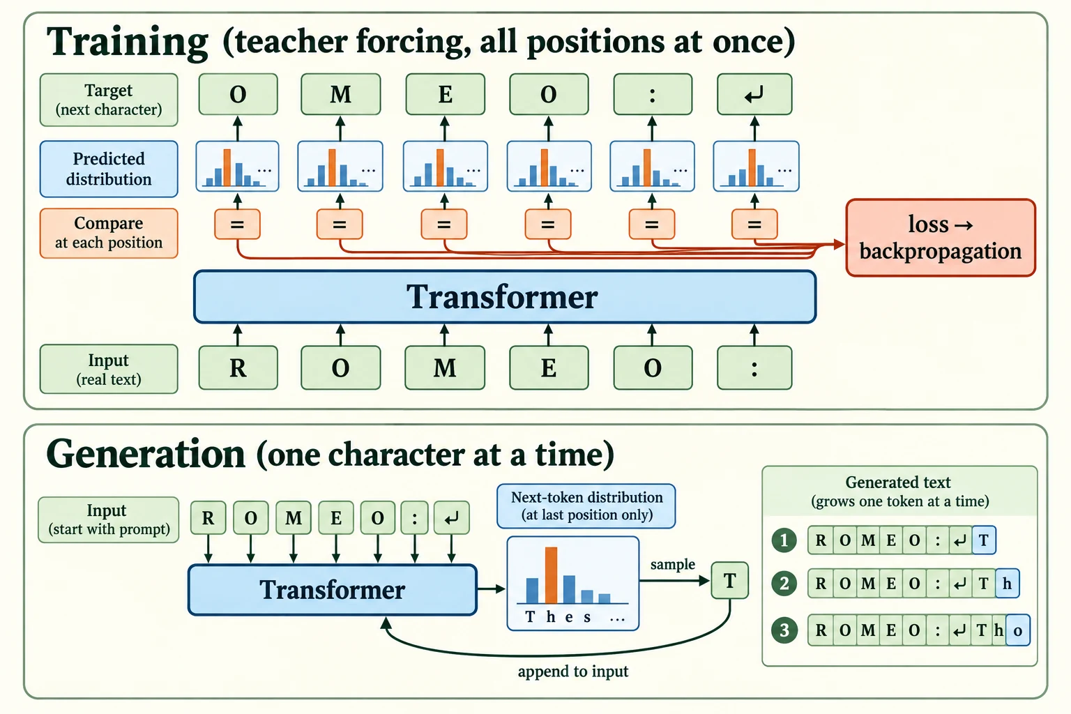
Figure 6.6.1. Teacher forcing compares every position with its true next character in one masked pass. Generation samples from the last position, appends the choice, and repeats with fixed weights. ↵ denotes a newline; the sample text is illustrative.
The first half of this lesson (Sections 2–7) is about training; the second half (Sections 8–10) is about generation.
PATH = "data/shakespeare/input.txt"os.makedirs("data/shakespeare", exist_ok=True)if not os.path.exists(PATH): urllib.request.urlretrieve("https://raw.githubusercontent.com/karpathy/char-rnn/master/data/tinyshakespeare/input.txt", PATH)text = open(PATH, encoding="utf-8").read()chars = sorted(set(text)); V = len(chars)stoi = {c: i for i, c in enumerate(chars)}; itos = {i: c for c, i in stoi.items()}encode = lambda s: [stoi[c] for c in s]; decode = lambda ids: "".join(itos[i] for i in ids)data = torch.tensor(encode(text), dtype=torch.long)n = int(0.9 * len(data)); train_ids, val_ids = data[:n], data[n:]CONTEXT, BATCH = 64, 32def get_batch(split, generator, batch_size=BATCH): """Sample input windows and their one-position-shifted targets; return two integer tensors. Arguments: split: Training or validation corpus selector. generator: Seeded generator for sampling. batch_size: Number of windows sampled per batch. """ d = train_ids if split == "train" else val_ids s = torch.randint(0, len(d) - CONTEXT - 1, (batch_size,), generator=generator) return torch.stack([d[i:i + CONTEXT] for i in s]), torch.stack([d[i + 1:i + CONTEXT + 1] for i in s])class CausalSelfAttention(nn.Module): """Projected multi-head self-attention with a causal mask and output projection.""" def __init__(self, d_model, n_heads): """Create the components of this model; the forward computation is traced in the lesson. Arguments: d_model: Feature width of each token vector. n_heads: Number of attention heads; divides model width. """ super().__init__() self.n_heads = n_heads self.qkv = nn.Linear(d_model, 3 * d_model); self.proj = nn.Linear(d_model, d_model) def forward(self, x): """Projected multi-head self-attention with a causal mask and output projection. Arguments: x: Floating-point tensor; image models use (B, C, H, W), token-vector models use (B, T, D). """ B, T, D = x.shape q, k, v = self.qkv(x).split(D, dim=2) q, k, v = [t.view(B, T, self.n_heads, D // self.n_heads).transpose(1, 2) for t in (q, k, v)] return self.proj(F.scaled_dot_product_attention(q, k, v, is_causal=True).transpose(1, 2).reshape(B, T, D))class Block(nn.Module): """Attention and feed-forward sub-layers with normalisation and residual additions.""" def __init__(self, d_model, n_heads): """Create the components of this model; the forward computation is traced in the lesson. Arguments: d_model: Feature width of each token vector. n_heads: Number of attention heads; divides model width. """ super().__init__() self.ln1, self.ln2 = nn.LayerNorm(d_model), nn.LayerNorm(d_model) self.attn = CausalSelfAttention(d_model, n_heads) self.ffn = nn.Sequential(nn.Linear(d_model, 4 * d_model), nn.GELU(), nn.Linear(4 * d_model, d_model)) def forward(self, x): """Attention and feed-forward sub-layers with normalisation and residual additions. Arguments: x: Floating-point tensor; image models use (B, C, H, W), token-vector models use (B, T, D). """ x = x + self.attn(self.ln1(x)) return x + self.ffn(self.ln2(x))class GPT(nn.Module): """Character-level decoder-only Transformer returning vocabulary logits and optional next-token loss.""" def __init__(self, vocab_size, d_model=64, n_heads=4, n_layers=3, context=CONTEXT): """Create the components of this model; the forward computation is traced in the lesson. Arguments: vocab_size: Number of token IDs represented by the embedding table. d_model: Feature width of each token vector. n_heads: Number of attention heads; divides model width. n_layers: Number of Transformer blocks. context: Maximum input-window length in tokens. """ super().__init__() self.context = context self.tok_emb, self.pos_emb = nn.Embedding(vocab_size, d_model), nn.Embedding(context, d_model) self.blocks = nn.ModuleList([Block(d_model, n_heads) for _ in range(n_layers)]) self.ln_f, self.head = nn.LayerNorm(d_model), nn.Linear(d_model, vocab_size) def forward(self, ids, targets=None): """Character-level decoder-only Transformer returning vocabulary logits and optional next-token loss. Arguments: ids: Integer token IDs, usually shaped (batch, tokens). targets: Optional next-token integer targets aligned with the input positions. """ x = self.tok_emb(ids) + self.pos_emb(torch.arange(ids.shape[1])) for b in self.blocks: x = b(x) logits = self.head(self.ln_f(x)) loss = None if targets is None else F.cross_entropy(logits.view(-1, logits.shape[-1]), targets.view(-1)) return logits, lossprint("training tokens:", len(train_ids), "| validation tokens:", len(val_ids), "| vocabulary:", V)print("model parameters:", sum(p.numel() for p in GPT(V).parameters()))training tokens: 1003854 | validation tokens: 111540 | vocabulary: 65 model parameters: 162561
The model and data are exactly as before: 1,003,854 training characters, 111,540 validation characters, a 65-character vocabulary, and a model with 162,561 parameters.
What differs between the training and generation loops?
Training uses known histories and updates weights; generation chooses tokens from its evolving history.
Next-Token Prediction
A language model is trained on one deceptively simple task: given the text so far, predict the next token. No labels are needed beyond the text itself; every character in the training data is the answer to the question "what comes after the characters before it?". This makes language modelling self-supervised, like the skip-gram objective in Lesson 5.3, and it is why language models can learn from enormous amounts of raw text.
Why should such a simple task produce anything impressive? Because predicting the next character well requires a lot of knowledge. To predict that "KING RICH" continues with "A", the model must have learned character names. To predict a line break followed by a speaker's name in capitals, it must have learned the layout of a play. To predict the end of a word it has never seen in exactly that context, it must have learned spelling patterns. Every regularity in the text becomes a way to reduce the loss. Large language models are trained on exactly this task, with subword tokens and vastly more text, and the knowledge they show is a by-product of predicting the next token very well.
Why is next-token prediction self-supervised?
The text supplies the targets without separately annotated labels.
Training Targets and Label Shifting
As we set up in Lesson 6.2, each training example is a window of text x and a target y that is the same window shifted one position to the left, so that y[t] is the character that follows x[t].
x, y = get_batch("train", torch.Generator().manual_seed(0), batch_size=1)print("input :", repr(decode(x[0, :24].tolist())))print("target:", repr(decode(y[0, :24].tolist())))print("target equals input shifted by one?", torch.equal(x[0, 1:], y[0, :-1]))input : 't, for his purpose in th' target: ', for his purpose in the' target equals input shifted by one? True
The input begins 't, for his purpose in th' and the target begins one character later, ', for his purpose in the'. The check confirms that the target is exactly the input shifted by one (True). Combined with the causal mask, this shift turns one window into many separate questions: at position t, "having seen x[0] to x[t], what is y[t]?".
What happens if targets are accidentally identical to inputs?
A causally masked model can learn an easy copying task.
Cross-Entropy Loss for Language Modelling
At each position, the model outputs a probability distribution over the 65 characters. The loss at that position is −log(the probability the model gave to the correct next character), and the overall loss is the average over all positions. This is the same cross-entropy loss you have used for classification since Module 1; a language model is simply a 65-way classifier applied at every position.
Here is a single position worked by hand, with three possible tokens:
logits = torch.tensor([2.0, 1.0, 0.1])target = 0probs = F.softmax(logits, dim=0)print("probabilities:", [round(v, 3) for v in probs.tolist()])print("loss by hand, -log p(target):", round(-math.log(probs[target].item()), 4))print("F.cross_entropy: ", round(F.cross_entropy(logits.unsqueeze(0), torch.tensor([target])).item(), 4))for p in [0.9, 0.5, 0.1, 0.01]: print(f"probability on the correct token {p:<4} -> loss {-math.log(p):.3f}")probabilities: [0.659, 0.242, 0.099] loss by hand, -log p(target): 0.417 F.cross_entropy: 0.417 probability on the correct token 0.9 -> loss 0.105 probability on the correct token 0.5 -> loss 0.693 probability on the correct token 0.1 -> loss 2.303 probability on the correct token 0.01 -> loss 4.605
Softmax turns the logits [2.0, 1.0, 0.1] into probabilities [0.659, 0.242, 0.099]. The correct token is the first, so the loss is −log(0.659) = 0.417, which matches F.cross_entropy. The table underneath shows how the loss depends on the probability given to the correct token: 0.105 at a probability of 0.9, 0.693 at 0.5, 2.303 at 0.1 and 4.605 at 0.01. The loss punishes confident mistakes severely and rewards confident correct answers.
4.1 Baselines: what does a given loss mean?
A loss of, say, 2.0 means nothing on its own. Before training, we compute the validation loss of three very simple predictors, which give us a scale to read our model's loss against:
- Uniform: every character equally likely.
- Character frequencies (unigram): always predict each character with its overall frequency in the training text, ignoring context entirely.
- Previous character only (bigram): predict the next character from the counts of which character follows which in the training text. This uses exactly one character of context.
counts_uni = torch.bincount(train_ids, minlength=V).float() + 1p_uni = counts_uni / counts_uni.sum()counts_bi = torch.ones(V, V) # add-one smoothingcounts_bi.index_put_((train_ids[:-1], train_ids[1:]), torch.ones(len(train_ids) - 1), accumulate=True)p_bi = counts_bi / counts_bi.sum(1, keepdim=True) # P(next | current)val_uniform = math.log(V)val_unigram = -p_uni[val_ids[1:]].log().mean().item()val_bigram = -p_bi[val_ids[:-1], val_ids[1:]].log().mean().item()print(f"validation loss, uniform guess: {val_uniform:.3f}")print(f"validation loss, character frequencies (unigram): {val_unigram:.3f}")print(f"validation loss, previous character only (bigram): {val_bigram:.3f}")print("bigram's most likely character after 'q':", repr(itos[p_bi[stoi['q']].argmax().item()]), f"(probability {p_bi[stoi['q']].max():.3f})")validation loss, uniform guess: 4.174 validation loss, character frequencies (unigram): 3.347 validation loss, previous character only (bigram): 2.482 bigram's most likely character after 'q': 'u' (probability 0.898)
On the validation text, a uniform guess scores 4.174, character frequencies 3.347, and the bigram model 2.482. The bigram model has already learned some real structure: after q, it predicts u with probability 0.898. Our Transformer sees up to 64 characters of context, so to be worth anything it must beat 2.482 clearly.
Key terms
- Next-token prediction: the task of predicting each token from the tokens before it.
- Self-supervised learning: learning from targets created from the data itself, here the next character.
- Unigram / bigram model: a predictor using no context / only the previous token.
-
A model gives the correct next character a probability of 0.25. What is its loss at that position?
−log(0.25) = log(4) ≈ 1.386.
Why compare validation loss with a bigram baseline?
It checks whether a complex model adds value beyond one-token context.
Teacher Forcing and Parallel Training
During training, the model always predicts each position from the real previous characters, never from its own earlier predictions. If it predicted the wrong character at position 5, position 6 still sees the true character at position 5. This is called teacher forcing: like a teacher correcting a student after every word, the model is always given the right history.
Teacher forcing has a huge practical benefit. Because the inputs at every position are known in advance (they are just the real text), the model does not have to wait for its own predictions, so all positions can be computed at once. Together with the causal mask, one forward pass gives a prediction and a loss term at every position in every window.
xb, yb = get_batch("train", torch.Generator().manual_seed(0))print("one batch:", tuple(xb.shape), "->", xb.numel(), "next-token predictions from a single forward pass")one batch: (32, 64) -> 2048 next-token predictions from a single forward pass
A batch of shape (32, 64) gives 2,048 next-character predictions from a single forward pass. A recurrent network would have to process the 64 positions one after another; a Transformer computes them all together. This parallelism is one of the main reasons Transformers could be trained on far more data than their predecessors.
Teacher forcing also has a cost, which we will meet in Section 10: at generation time there is no teacher, and the model must live with its own mistakes.
Key terms
- Teacher forcing: during training, feeding the model the true previous tokens rather than its own predictions.
- Parallel training: computing predictions and losses for all positions in one forward pass.
Why does teacher forcing permit parallel training predictions?
All input histories are known, with future visibility blocked by the causal mask.
Training Stability: AdamW, Warmup, Schedules and Clipping
The training function below brings together four tools you have met in Module 3 and Lesson 6.4:
- AdamW is Adam with decoupled weight decay: a small pull of every weight towards zero, applied separately from the gradient update, which acts as regularisation. It is the standard optimizer for Transformers.
- Learning-rate warmup raises the learning rate linearly from almost zero over the first 100 steps, so the first, most chaotic updates are small. In Lesson 6.4 it was the difference between a post-norm model that collapsed and one that trained.
- Cosine decay then lowers the learning rate smoothly from its peak to zero, following half a cosine wave. Large steps early let the model make fast progress; small steps late let it settle into a good solution.
- Gradient clipping rescales the gradients whenever their overall size (norm) exceeds a threshold, here 1.0, so that one unusual batch cannot produce a huge, damaging update.
clip_grad_norm_also returns the norm before clipping, which we record as a health check.
We also prepare 10 fixed validation batches, so that every validation loss is measured on exactly the same 640 windows.
VAL_BATCHES = [get_batch("val", torch.Generator().manual_seed(1000 + i), batch_size=64) for i in range(10)]@torch.no_grad()def val_loss(model): """Average loss on the fixed validation batches without gradients, then restore training mode. Arguments: model: Model being trained, evaluated or inspected. """ model.eval() out = np.mean([model(xv, yv)[1].item() for xv, yv in VAL_BATCHES]) model.train() return outdef lr_at(step, peak, steps, warmup): """Compute the warmup/cosine learning rate at a zero-based training step. Arguments: step: Zero-based optimiser update index. peak: Peak learning rate. steps: Number of optimiser updates. warmup: Number of initial learning-rate warmup steps. """ if step < warmup: return peak * (step + 1) / warmup # linear warmup progress = (step - warmup) / max(1, steps - warmup) return peak * 0.5 * (1 + math.cos(math.pi * progress)) # cosine decay to zerodef train(peak_lr, steps, warmup=0, schedule=True, clip=1.0, seed=0, eval_every=None): """Train with the declared split, optimiser and budget; return the measurements described at the call site. Arguments: peak_lr: Peak learning rate. steps: Number of optimiser updates. warmup: Number of initial learning-rate warmup steps. schedule: Whether to use the warmup/cosine schedule rather than a constant rate. clip: Threshold for the combined gradient norm. seed: Random seed for this experiment. eval_every: Interval between validation measurements. """ torch.manual_seed(seed) model = GPT(V) opt = torch.optim.AdamW(model.parameters(), lr=peak_lr, weight_decay=0.01) g = torch.Generator().manual_seed(seed) log = {"train": [], "grad_norm": [], "lr": [], "val": []} for step in range(steps): lr = lr_at(step, peak_lr, steps, warmup) if schedule else peak_lr for group in opt.param_groups: group["lr"] = lr x, y = get_batch("train", g) _, loss = model(x, y) opt.zero_grad(set_to_none=True) loss.backward() norm = torch.nn.utils.clip_grad_norm_(model.parameters(), clip) # returns the norm BEFORE clipping opt.step() log["train"].append(loss.item()); log["grad_norm"].append(norm.item()); log["lr"].append(lr) if eval_every and ((step + 1) % eval_every == 0): log["val"].append((step + 1, val_loss(model))) return model, logHere is the learning-rate schedule we will use for the main run: a straight climb to the peak over 100 steps, then a smooth cosine descent to zero at step 1,400.
steps = np.arange(1400)plt.figure(figsize=(6.5, 3.2))plt.plot(steps, [lr_at(s, 1e-2, 1400, 100) for s in steps])plt.xlabel("training step"); plt.ylabel("learning rate"); plt.title("Linear warmup (100 steps), then cosine decay")plt.grid(alpha=0.3); plt.tight_layout(); plt.show()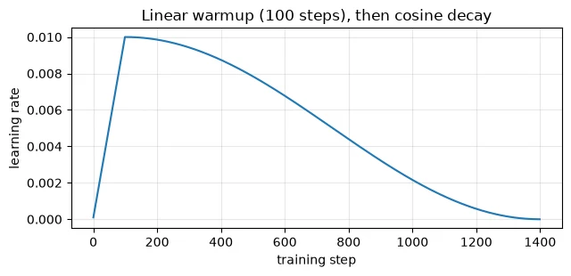
6.1 Choosing the learning rate on validation
The peak learning rate is the most important setting to get right, so we choose it with a short experiment: train for 200 steps at three learning rates, with a constant learning rate and no warmup, and compare the validation loss. We never use the validation data to compute gradients, and we use the same random batches for every run.
sweep = {}for lr in [1e-3, 3e-3, 1e-2]: m, _ = train(lr, steps=200, warmup=0, schedule=False) sweep[lr] = val_loss(m) print(f"peak learning rate {lr:<6}: validation loss after 200 steps {sweep[lr]:.3f}")best_lr = min(sweep, key=sweep.get)print("chosen on validation:", best_lr)peak learning rate 0.001 : validation loss after 200 steps 2.489 peak learning rate 0.003 : validation loss after 200 steps 2.330 peak learning rate 0.01 : validation loss after 200 steps 2.190 chosen on validation: 0.01
After 200 steps, a learning rate of 0.001 reaches a validation loss of 2.489, 0.003 reaches 2.330 and 0.01 reaches 2.190. The highest learning rate wins, so we choose 0.01.
A caution about short sweeps: they favour higher learning rates, because a larger step size makes faster progress early on, even if it might cause trouble later. That is one reason we pair the chosen rate with warmup and decay, and why we check the full run's curves rather than trusting the sweep blindly.
Common mistake: choosing settings by looking at the test set, or at the training loss. Training loss rewards memorisation; the test set must stay untouched until the very end. Choose on validation.
What does gradient clipping at norm 1 do?
Rescale gradients only when their combined norm exceeds 1.
Training on Tiny Shakespeare and Reading the Loss Curves
Now the main run: 1,400 steps with a peak learning rate of 0.01, 100 warmup steps, cosine decay, AdamW and clipping at 1.0. Every 100 steps, we measure the validation loss. We also keep a copy of the untrained model for comparison.
STEPS, WARMUP = 1400, 100torch.manual_seed(0); untrained = GPT(V) # a copy of the starting point, for comparisons latermodel, log = train(best_lr, STEPS, warmup=WARMUP, eval_every=100)print("validation loss every 100 steps:", [round(float(v), 3) for _, v in log["val"]])print(f"final validation loss: {log['val'][-1][1]:.3f}")print(f"average training loss over the last 100 steps: {np.mean(log['train'][-100:]):.3f}")validation loss every 100 steps: [2.487, 2.222, 2.111, 2.006, 1.95, 1.906, 1.864, 1.845, 1.805, 1.788, 1.765, 1.752, 1.744, 1.742] final validation loss: 1.742 average training loss over the last 100 steps: 1.547
The validation loss falls steadily, from 2.487 after 100 steps to 1.742 at the end. It is still creeping down at the end, but slowly: the last three measurements are 1.752, 1.744 and 1.742, as the cosine schedule brings the learning rate down to zero. The average training loss over the last 100 steps is 1.547. Let's look at the curves, together with the gradient norms.
fig, axes = plt.subplots(1, 2, figsize=(12, 4))sm = np.convolve(log["train"], np.ones(25) / 25, mode="valid")axes[0].plot(log["train"], alpha=0.25, color="tab:blue", label="training loss (each step)")axes[0].plot(np.arange(24, STEPS), sm, color="tab:blue", label="training loss (25-step average)")axes[0].plot(*zip(*log["val"]), "o-", color="tab:orange", label="validation loss")for v_, name in [(val_unigram, "character frequencies"), (val_bigram, "bigram")]: axes[0].axhline(v_, ls="--", lw=1, color="grey"); axes[0].text(STEPS * 0.62, v_ + 0.03, name, fontsize=8, color="grey")axes[0].set_xlabel("step"); axes[0].set_ylabel("loss"); axes[0].set_ylim(1.4, 4.5); axes[0].legend(fontsize=8)axes[0].set_title("Loss curves"); axes[0].grid(alpha=0.3)axes[1].plot(log["grad_norm"], lw=0.8); axes[1].axhline(1.0, color="red", ls="--", lw=1, label="clipping threshold")axes[1].set_yscale("log"); axes[1].set_xlabel("step"); axes[1].set_ylabel("gradient norm before clipping (log)")axes[1].set_title("Gradient norms"); axes[1].legend(fontsize=8); axes[1].grid(alpha=0.3)plt.tight_layout(); plt.show()gn = np.array(log["grad_norm"])print(f"steps where clipping was active (norm above 1.0): {(gn > 1.0).sum()} of {STEPS}")print(f"largest gradient norm: {gn.max():.2f} (at step {gn.argmax()}) | median: {np.median(gn):.2f}")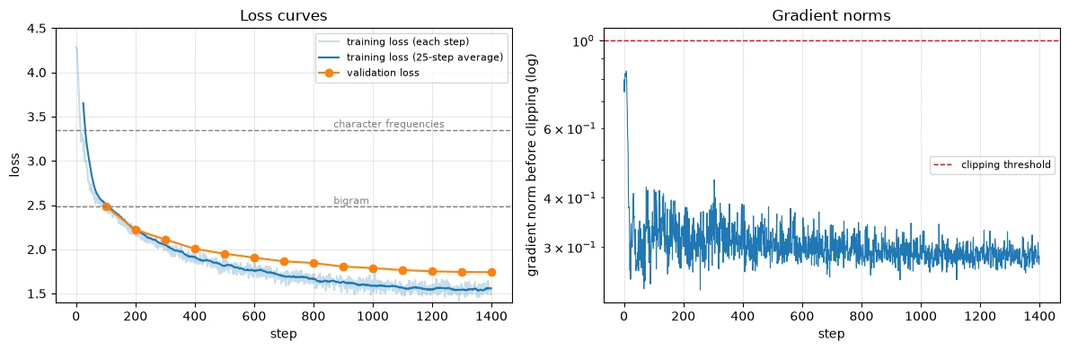
steps where clipping was active (norm above 1.0): 0 of 1400
largest gradient norm: 0.84 (at step 8) | median: 0.30
Reading the loss curves (left). Start with the baselines. The model passes the character-frequency baseline (3.347) almost immediately, and the bigram baseline (2.482) at about step 100, where its validation loss is 2.487. From there on it is using more than one character of context. It ends at 1.742, far below the bigram's 2.482.
Notice the growing gap between training loss (1.547 at the end) and validation loss (1.742). The model does somewhat better on the plays it trained on than on the held-out ones, but both curves are still falling together, with no sign of the validation loss turning upwards. This is a generalisation gap. There is no observed validation upturn in this run, although that alone cannot rule out all overfitting: in Module 3's terms, "train ↓, validation ↓".
Reading the gradient norms (right). The gradient norm starts high in the first few steps, peaking at 0.84 at step 8, then settles around a median of 0.30. It never reaches the clipping threshold of 1.0: clipping was active on 0 of 1,400 steps. In this run, with pre-norm blocks and warmup, clipping turned out to be unnecessary. That is typical of a healthy run: clipping is insurance, which only matters when a bad batch or an unstable setup produces a spike like the 117.6 in Lesson 6.4's collapsed post-norm run. It costs almost nothing to keep.
7.1 What did the model learn?
Let's compare the untrained and trained models' predictions after a few prompts.
@torch.no_grad()def next_distribution(model, prompt): """Return last-position vocabulary logits for the prompt's retained context. Arguments: model: Model being trained, evaluated or inspected. prompt: Nonempty known-character text prefix. """ model.eval() logits, _ = model(torch.tensor([encode(prompt[-CONTEXT:])])) return logits[0, -1] # scores for the next characterprompts = ["First Citiz", "KING RICH", "What light through yonder windo", "my good lor"]for prompt in prompts: for name, m in [("untrained", untrained), ("trained", model)]: p = F.softmax(next_distribution(m, prompt), dim=-1) top = p.topk(3) print(f"{name:<9} after {prompt!r:<34} top 3 =", [(repr(itos[i.item()]), round(v.item(), 3)) for v, i in zip(top.values, top.indices)])untrained after 'First Citiz' top 3 = [("'W'", 0.042), ("'P'", 0.035), ("'\\n'", 0.031)]
trained after 'First Citiz' top 3 = [("'e'", 0.966), ("'i'", 0.013), ("'o'", 0.006)]
untrained after 'KING RICH' top 3 = [("'t'", 0.05), ("'n'", 0.041), ("'S'", 0.037)]
trained after 'KING RICH' top 3 = [("'A'", 0.986), ("'M'", 0.003), ("'E'", 0.003)]
untrained after 'What light through yonder windo' top 3 = [("'u'", 0.042), ("'g'", 0.042), ("'G'", 0.035)]
trained after 'What light through yonder windo' top 3 = [("'m'", 0.396), ("'n'", 0.353), ("'w'", 0.069)]
untrained after 'my good lor' top 3 = [("'t'", 0.042), ("'u'", 0.038), ("'h'", 0.035)]
trained after 'my good lor' top 3 = [("'d'", 0.993), ("'s'", 0.001), ("'y'", 0.001)]
The untrained model's best guesses are random, around 0.04 to 0.05 each. The trained model is confident and usually right:
- After "First Citiz" it predicts
'e'with probability 0.966: it knows the speaker name "First Citizen". - After "KING RICH" it predicts
'A'with 0.986: it knows "KING RICHARD", written in capitals. - After "my good lor" it predicts
'd'with 0.993.
But not always. After "What light through yonder windo" its top guesses are 'm' (0.396) and 'n' (0.353), and the correct 'w' gets only 0.069. "Window" is rare in this text, and a small model trained for a couple of minutes has not learned it; "windom" and "window" might be equally plausible to it as spellings. Its knowledge is real but patchy.
7.2 How much context does the model use?
The model sees up to 64 characters, but how much does it actually benefit from them? We can measure the validation loss separately at each position in the window: at position 0 the model has seen only one character, at position 63 it has seen 64.
@torch.no_grad()def loss_by_position(m): """Average validation cross-entropy by position; targets differ between positions, so this is not a controlled context ablation. Arguments: m: Model being evaluated. """ m.eval() per_pos = torch.zeros(CONTEXT) for xv, yv in VAL_BATCHES: logits, _ = m(xv) per_pos += F.cross_entropy(logits.transpose(1, 2), yv, reduction="none").mean(0) # (64,) one loss per position return (per_pos / len(VAL_BATCHES)).numpy()lp_trained, lp_untrained = loss_by_position(model), loss_by_position(untrained)for pos in [0, 1, 2, 4, 8, 16, 32, 63]: print(f"position {pos:>2} (sees {pos + 1:>2} characters): trained validation loss {lp_trained[pos]:.3f}")plt.figure(figsize=(6.5, 3.6))plt.plot(lp_untrained, label="untrained"); plt.plot(lp_trained, label="trained")plt.axhline(val_unigram, color="grey", ls="--", lw=1, label="character frequencies")plt.axhline(val_bigram, color="grey", ls=":", lw=1, label="bigram")plt.xlabel("position in the window (= characters of context - 1)"); plt.ylabel("validation loss")plt.title("More context helps, mostly in the first few characters"); plt.legend(fontsize=8); plt.grid(alpha=0.3); plt.tight_layout(); plt.show()position 0 (sees 1 characters): trained validation loss 2.424 position 1 (sees 2 characters): trained validation loss 2.196 position 2 (sees 3 characters): trained validation loss 1.952 position 4 (sees 5 characters): trained validation loss 1.794 position 8 (sees 9 characters): trained validation loss 1.712 position 16 (sees 17 characters): trained validation loss 1.663 position 32 (sees 33 characters): trained validation loss 1.770 position 63 (sees 64 characters): trained validation loss 1.748
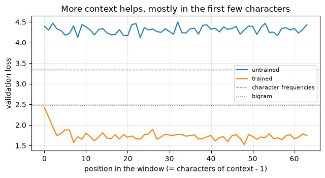
At position 0, with just one character to go on, the validation loss is 2.424, close to the bigram model's 2.482. That makes sense: with one character of context, the Transformer can do little more than a bigram model. The loss falls quickly as context grows: 2.196 with 2 characters, 1.952 with 3, 1.794 with 5 and 1.712 with 9. After that, the curve flattens out at roughly 1.7, with some noise from position to position: 1.663 at position 16, 1.770 at 32 and 1.748 at 63.
Loss improves rapidly over the first few positions and then levels off in this diagnostic. This is consistent with useful short context, but it does not establish that the model ignores everything beyond ten characters: different positions predict different targets and use different learned position vectors. A controlled context-length test should predict the same held-out target tokens with progressively truncated histories. Longer-range ability depends on the data, training, architecture and task.
7.3 Inside the trained attention
In Lesson 6.3 we built, by hand, a head that attends to the previous token. Did training produce anything similar? Here are the attention weights of the four heads in the first block for the line "KING RICHARD:\nThe king is dead", with numbers summarising, for each head, how much weight goes to each distance back.
@torch.no_grad()def attention_weights(model, text_, layer): """Recompute causal attention weights for one selected block and input line. Arguments: model: Model being trained, evaluated or inspected. text_: Input line to inspect. layer: Zero-based Transformer block index. """ ids = torch.tensor([encode(text_)]) x = model.tok_emb(ids) + model.pos_emb(torch.arange(ids.shape[1])) for i, b in enumerate(model.blocks): if i == layer: h = b.ln1(x); B, T, D = h.shape; H = b.attn.n_heads q, k, _ = b.attn.qkv(h).split(D, dim=2) q, k = [t.view(B, T, H, D // H).transpose(1, 2) for t in (q, k)] s = q @ k.transpose(-2, -1) / math.sqrt(D // H) return torch.softmax(s.masked_fill(~torch.tril(torch.ones(T, T, dtype=torch.bool)), float("-inf")), -1)[0] x = b(x)line = "KING RICHARD:\nThe king is dead"model.eval()w0 = attention_weights(model, line, layer=0)labels = [repr(c)[1:-1] if c != " " else "␣" for c in line]fig, axes = plt.subplots(1, 4, figsize=(15, 4.4))for h, ax in enumerate(axes): ax.imshow(w0[h], cmap="Blues", vmin=0, vmax=1) ax.set_xticks(range(len(line)), labels, fontsize=6); ax.set_yticks(range(len(line)), labels, fontsize=6) ax.set_title(f"trained model, block 1, head {h}", fontsize=9)plt.tight_layout(); plt.show()T_ = len(line)print("average attention weight at each distance back (0 = itself, 1 = previous character, ...):")for h in range(4): prof = [np.mean([w0[h, i, i - d].item() for i in range(d, T_)]) for d in range(4)] print(f" head {h}: " + " ".join(f"{d} back: {v:.2f}" for d, v in enumerate(prof)))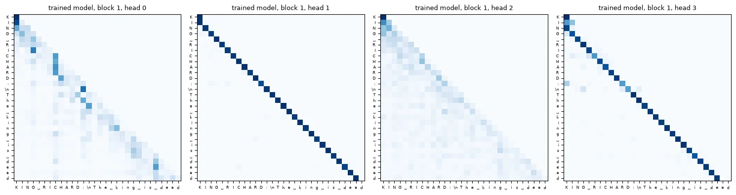
average attention weight at each distance back (0 = itself, 1 = previous character, ...):
  head 0: 0 back: 0.12  1 back: 0.20  2 back: 0.18  3 back: 0.24
  head 1: 0 back: 0.04  1 back: 0.97  2 back: 0.00  3 back: 0.00
  head 2: 0 back: 0.13  1 back: 0.20  2 back: 0.10  3 back: 0.12
  head 3: 0 back: 0.06  1 back: 0.03  2 back: 0.91  3 back: 0.03
Two heads have learned sharp positional rules entirely on their own:
- Head 1 puts an average weight of 0.97 on the previous character: it is the "previous token" head we designed by hand in Lesson 6.3, discovered by training.
- Head 3 puts 0.91 on the character two positions back.
Together, they let the next block see the last three characters directly. Heads 0 and 2 spread their attention more widely over the recent past (no more than 0.24 on any single distance in the first few), gathering broader context. Compare these sharp, purposeful patterns with the noisy weights of the untrained module in Lesson 6.3.
Common mistake: reading too much into a single attention map. Attention shows where information is gathered from, not what is done with it, and later blocks may change everything. Here we backed the pictures with averages over a whole line; for real conclusions, measure over many inputs.
Does a flat loss-by-position curve prove that all longer context is ignored?
No; test the same target tokens under controlled history truncations.
Autoregressive Inference
Now the second half: generation. A trained model gives us a probability distribution for the next character. To write text, we repeat four steps:
- Run the model on the text so far (at most the last 64 characters, the context window).
- Take the logits at the last position only: the model's scores for the next character.
- Choose a character from them. Section 9 is about how.
- Append it to the text, and go back to step 1.
This is called autoregressive generation: each new token is predicted from the model's own previous outputs. Here is the full function, with the choice step written to support all the strategies of Section 9, followed by 300 characters generated after the prompt "ROMEO:" by sampling from the model's distribution as it is.
@torch.no_grad()def generate(model, prompt, n_new, temperature=1.0, top_k=None, top_p=None, seed=0): """Generate additional characters autoregressively from the prompt; return the prompt and continuation. Arguments: model: Model being trained, evaluated or inspected. prompt: Nonempty known-character text prefix. n_new: Number of new characters to append. temperature: Positive logit divisor; zero selects greedy decoding in this implementation. top_k: Optional number of highest-scoring candidate tokens to retain. top_p: Optional cumulative-probability threshold for nucleus sampling. seed: Random seed for this experiment. """ model.eval() g = torch.Generator().manual_seed(seed) ids = encode(prompt) for _ in range(n_new): logits = next_distribution(model, decode(ids)) # 1. run the model on the text so far if temperature == 0: # greedy: always the single most likely token ids.append(int(logits.argmax())); continue logits = logits / temperature # 2. sharpen (<1) or flatten (>1) if top_k is not None: # 3a. keep only the k most likely tokens kth = logits.topk(top_k).values[-1] logits = logits.masked_fill(logits < kth, float("-inf")) if top_p is not None: # 3b. keep the smallest set with total probability >= p sorted_logits, order = logits.sort(descending=True) cum = F.softmax(sorted_logits, -1).cumsum(-1) drop = cum - F.softmax(sorted_logits, -1) >= top_p logits[order[drop]] = float("-inf") probs = F.softmax(logits, dim=-1) ids.append(int(torch.multinomial(probs, 1, generator=g))) # 4. draw the next token return decode(ids)print(generate(model, "ROMEO:\n", 300, temperature=1.0, seed=0))ROMEO: Thy for this when? I would nextand, in I to thee, Is upon his thee rechest of bleepelies. To him; that's your wake excheeksiard; Her none have too we woot to a man is hither. DORK: BUCKINGHRMOP. QUEEN MERSET: KINGHAM: Senatisarful too queen to this suild. JULIET: Farink'S yound, Englace that ha
Compare this with the random characters of the untrained model in Lesson 6.5. The trained model has learned the form of a play: speaker names in capitals followed by a colon and a line break ("JULIET:", "QUEEN MERSET:", "KINGHAM:"), lines of verse that start with capitals, punctuation in sensible places, and many real words ("I would", "to thee", "that's your", "a man is hither"). It has not learned meaning: the sentences do not make sense, and it invents words ("bleepelies", "excheeksiard") and names ("BUCKINGHRMOP"). For a 162,561-parameter model trained for a couple of minutes on one CPU core, reading one character at a time, that is about what we should expect.
Visual walkthrough: Follow the autoregressive loop.
Play or step through three character choices. Each chosen character becomes part of the next input; model weights stay fixed.
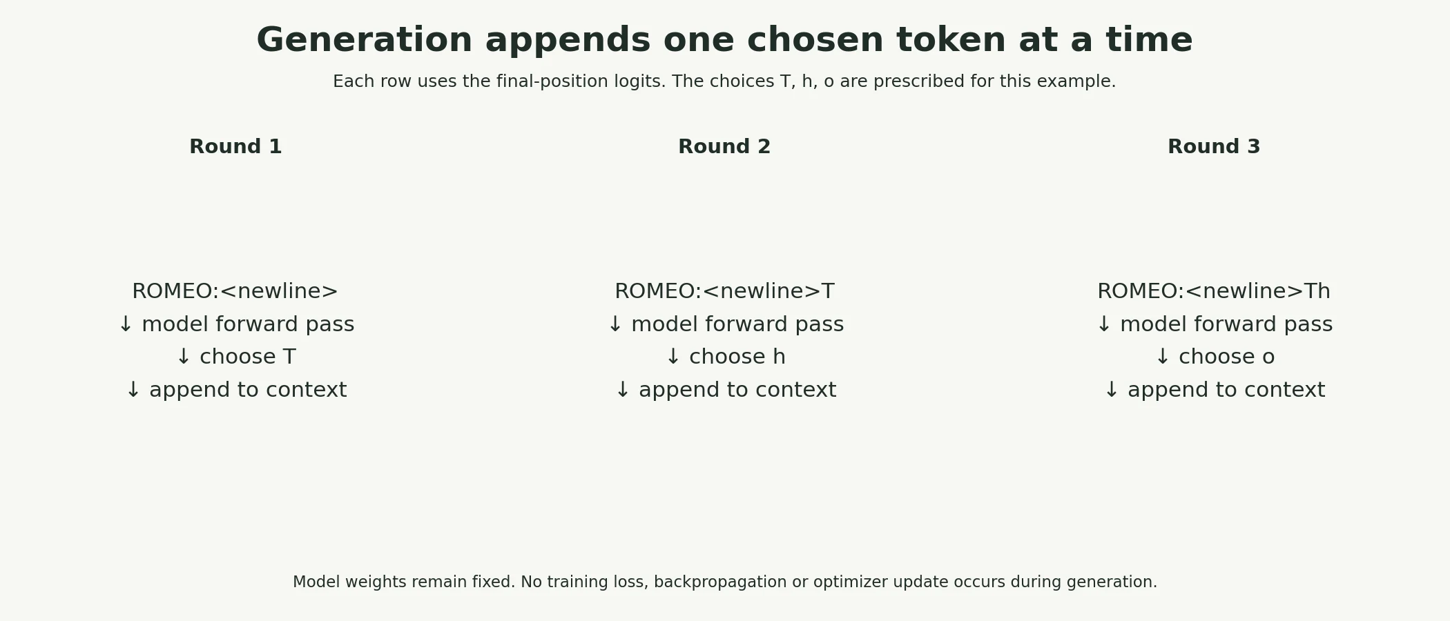
These supplied numbers illustrate the calculation. The web app adds a paused, step-by-step animation of the same example.
Paused on arrival. Use Previous step, Play/Pause, Next step or Reset. This is a fixed worked example, not a live trained model.
Which prediction is used to append a new generated token?
The vocabulary distribution at the last input position.
Greedy Decoding and Sampling
At step 3 of the generation loop, the model gives us a probability distribution, and we must turn it into a single choice. This choice, called the decoding strategy, has a big effect on the text.
- Greedy decoding always picks the single most likely token. It is deterministic: the same prompt always gives the same text.
- Sampling draws the next token at random according to the model's probabilities, so a token with probability 0.3 is chosen about 30% of the time.
Sampling is usually modified in one of three ways:
- Temperature. Divide the logits by a number T before softmax. T below 1 makes the distribution sharper (more confident); T above 1 makes it flatter (more adventurous); T = 1 leaves it unchanged; and T approaching 0 becomes greedy.
- Top-k. Keep only the k most likely tokens and set the rest to zero probability before sampling.
- Top-p (nucleus sampling). Keep the smallest set of most likely tokens whose probabilities add up to at least p, and drop the rest. Unlike top-k, the number of candidates adapts to how confident the model is.
Let's see temperature's effect on one real distribution: the model's prediction for the character after "...What light through yonder ".
logits = next_distribution(model, "ROMEO:\nWhat light through yonder ")fig, axes = plt.subplots(1, 3, figsize=(12, 3.2), sharey=True)for ax, t in zip(axes, [0.5, 1.0, 1.5]): p = F.softmax(logits / t, -1); top = p.topk(12) ax.bar([repr(itos[i.item()])[1:-1] or "␣" for i in top.indices], top.values.numpy()) ent = -(p * p.log()).sum().item() ax.set_title(f"temperature {t}: top prob {top.values[0]:.2f}, entropy {ent:.2f}", fontsize=9)axes[0].set_ylabel("probability"); plt.suptitle("Next-character distribution after '...through yonder '", fontsize=10)plt.tight_layout(); plt.show()for t in [0.5, 1.0, 1.5]: p_t = F.softmax(logits / t, -1) print(f"temperature {t}: top probability {p_t.max():.2f} for {repr(itos[p_t.argmax().item()])} | entropy {-(p_t * p_t.log()).sum():.2f}")p = F.softmax(logits, -1); sp = p.sort(descending=True).valuesprint("candidates kept by top-p 0.9 here:", int(((sp.cumsum(0) - sp) < 0.9).sum()), "| by top-k 5: 5")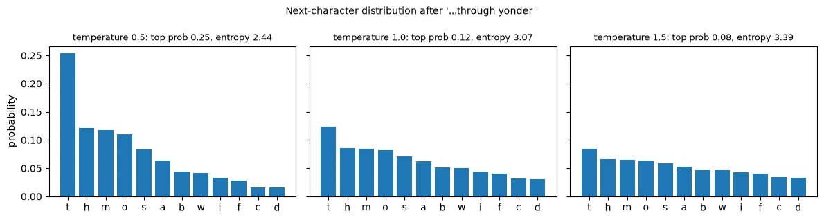
temperature 0.5: top probability 0.25 for 't' | entropy 2.44
temperature 1.0: top probability 0.12 for 't' | entropy 3.07
temperature 1.5: top probability 0.08 for 't' | entropy 3.39
candidates kept by top-p 0.9 here: 18 | by top-k 5: 5
At temperature 1.0 the most likely next character is 't' (as in "the" or "thy") with probability 0.12, with an entropy of 3.07. At temperature 0.5 the same distribution becomes much sharper, with 't' at 0.25 and the entropy down to 2.44. At 1.5 it flattens to 0.08 and 3.39. Temperature never changes the order of the candidates, only how strongly the model prefers the top ones. Here, top-p with p = 0.9 keeps 18 candidates, while top-k with k = 5 would keep exactly 5.
Now let's measure what each strategy does to the generated text. For each strategy we generate 300 characters after "ROMEO:", three times with different random seeds, and measure two things:
- Training-vocabulary words: the share of generated words that appear somewhere in the training text. This measures vocabulary coverage, not factuality, grammaticality or meaning.
- Distinct 8-character pieces: the share of all 8-character stretches of the output that are different from each other, a measure of variety. Text that repeats itself scores low.
train_words = set(re.findall(r"[A-Za-z']+", decode(train_ids.tolist())))def quality(sample, prompt_len): """Measure training-vocabulary word coverage and distinct 8-character spans; neither measures factuality. Arguments: sample: Generated text including its prompt. prompt_len: Number of initial characters excluded from generation metrics. """ words = re.findall(r"[A-Za-z']+", sample[prompt_len:]) real = np.mean([w in train_words for w in words]) if words else 0.0 grams = [sample[i:i + 8] for i in range(prompt_len, len(sample) - 8)] distinct = len(set(grams)) / max(1, len(grams)) return real, distinctsettings = [("greedy (temperature 0)", dict(temperature=0)), ("temperature 0.5", dict(temperature=0.5)), ("temperature 1.0", dict(temperature=1.0)), ("temperature 1.5", dict(temperature=1.5)), ("top-k, k = 5", dict(temperature=1.0, top_k=5)), ("top-p, p = 0.9", dict(temperature=1.0, top_p=0.9))]P0 = "ROMEO:\n"samples = {}print(f"{'decoding':<24} {'real words':>10} {'distinct 8-char pieces':>23}")for name, kw in settings: real, dist = [], [] for seed in range(3): s = generate(model, P0, 300, seed=seed, **kw) r, d = quality(s, len(P0)); real.append(r); dist.append(d) if seed == 0: samples[name] = s print(f"{name:<24} {np.mean(real):>10.3f} {np.mean(dist):>23.3f}")decoding real words distinct 8-char pieces greedy (temperature 0) 0.984 0.188 temperature 0.5 0.919 0.992 temperature 1.0 0.801 0.997 temperature 1.5 0.450 1.000 top-k, k = 5 0.869 1.000 top-p, p = 0.9 0.830 0.997
The trade-off is very clear:
| Decoding | Real words | Distinct 8-character pieces |
|---|---|---|
| Greedy | 0.984 | 0.188 |
| Temperature 0.5 | 0.919 | 0.992 |
| Temperature 1.0 | 0.801 | 0.997 |
| Temperature 1.5 | 0.450 | 1.000 |
| Top-k, k = 5 | 0.869 | 1.000 |
| Top-p, p = 0.9 | 0.830 | 0.997 |
Greedy decoding uses almost only real words (0.984), but only 0.188 of its 8-character pieces are distinct: it repeats itself. Raising the temperature trades training-vocabulary word coverage for variety in these samples: at 1.5, fewer than half the words are real (0.450). Top-k and top-p improve on plain sampling at temperature 1.0 (0.869 and 0.830 real words, against 0.801) without losing variety, because they cut off the long tail of unlikely characters, where most invented words come from. Here are some of the samples behind those numbers:
for name in ["greedy (temperature 0)", "temperature 0.5", "temperature 1.5", "top-p, p = 0.9"]: print(f"===== {name} =====") print(samples[name][:230]); print()===== greedy (temperature 0) ===== ROMEO: I am the shall the shall be some to the conter To the stand the shall the shall the shall the shall the shall the shall the shall the shall the shall the shall the shall the shall the shall the shall the shall the shall the ===== temperature 0.5 ===== ROMEO: There have the self made thee hand, And genemently of the countrest may the poor And serve the contents of or way we with that thou we never thee. LADY ANNE: I'll is he did the contring. First Marcius, I will not is the e ===== temperature 1.5 ===== ROMEO: thyre his khaxps: LeWToHat nexhand, in IgAlsternay oful you foth here hath Doigs Apeliess. I havest at's your wake excheeksiard; Her ne-days thysorrely you for 'falion? LEONTESS Lantsmuzen: Renjure a mother plain-will moon ===== top-p, p = 0.9 ===== ROMEO: Thou must therest triboural expace, And get the recome of his therefess the hight. First Gentleman: Who speak a pervace trucker, to not my father well. RIVERS: He seek, the he contring. FROMENES: How to faith and look, A
The greedy output falls into a loop almost immediately: "the shall the shall the shall..." over and over. Once the model has produced "the shall", the most likely continuation leads straight back to it, and greedy decoding has no way to escape. Temperature 0.5 reads most like English, with plausible phrases such as "serve the contents". Temperature 1.5 dissolves into invented words and stray capitals ("LeWToHat nexhand"). Top-p keeps the variety while producing a more convincing play layout.
There is no single best setting: it depends on the use. Lower temperature can make outputs more repeatable; more sampling can increase variety. Neither greedy decoding nor a low temperature guarantees factual accuracy. Our "real words" score only checks membership in the training vocabulary: repeated familiar words can still form meaningless or false sentences. Choose a strategy using evaluations appropriate to the task, including factuality when it matters.
Common mistake: concluding that a model is "broken" because greedy decoding produces endless repetition. Repetition loops are a known property of greedy decoding, not necessarily of the model. Try sampling with temperature, top-k or top-p before drawing conclusions.
Key terms
- Autoregressive generation: producing a sequence one token at a time, each predicted from the tokens generated so far.
- Decoding strategy: the rule for choosing a token from the model's distribution.
- Greedy decoding: always choosing the most likely token.
- Temperature: dividing logits by T before softmax; T < 1 sharpens, T > 1 flattens.
- Top-k / top-p sampling: sampling only from the k most likely tokens / from the smallest set covering probability p.
-
At temperature 0.5, the model's top probability after "...through yonder " rose from 0.12 to 0.25. What would you expect at temperature 0.1?
Dividing the logits by 0.1 multiplies the differences between them by 10, so the distribution becomes extremely sharp: almost all the probability would go to
't', and the result would be very close to greedy decoding.
Does greedy decoding guarantee factual answers?
No; it picks the most likely next token and can still be wrong or repetitive.
Training vs. Inference
Training and generation use the same model, but they differ in important ways:
| Training | Inference (generation) | |
|---|---|---|
| Input | Real text windows | The prompt plus the model's own output |
| Positions predicted | All of them at once (teacher forcing) | One new token per forward pass |
| Gradients | Computed (loss.backward()) |
Not needed (torch.no_grad()) |
| Model mode | model.train() |
model.eval() |
| Speed bottleneck | Total compute per batch | One forward pass per generated token |
Two of these differences show up directly in code:
model.train(); print("model.training after model.train():", model.training)model.eval(); print("model.training after model.eval(): ", model.training)with torch.no_grad(): _, l = model(*VAL_BATCHES[0])print("gradients tracked inside torch.no_grad()?", l.requires_grad)print("forward passes needed to generate 300 characters:", 300)model.training after model.train(): True model.training after model.eval(): False gradients tracked inside torch.no_grad()? False forward passes needed to generate 300 characters: 300
model.train() and model.eval() set the model's training flag (True and False). Our model has no dropout or batch normalisation, so the flag changes nothing here, but in models that have them it changes their behaviour, so the correct mode is a habit worth keeping (Module 2). Inside torch.no_grad(), the loss has requires_grad equal to False: PyTorch does not store anything for backpropagation, which saves memory and time during generation.
The last line points to the main cost of generation: 300 new characters need 300 separate forward passes, one after another. Training processes many positions in parallel, but generation is inherently sequential. Production systems speed this up with a KV cache, which stores the keys and values already computed for earlier tokens so that each new step only has to process the newest token. You will meet it again in Module 7.
The other important difference is exposure bias: during training the model always saw real text, but during generation it sees its own output, mistakes included. One invented word, such as "BUCKINGHRMOP", becomes part of the context for everything that follows, and the model was never trained to recover from its own errors. Sampling strategies that avoid unlikely tokens reduce this problem; they do not remove it.
Key terms
- Inference: using a trained model to make predictions, without updating its weights.
- KV cache: stored keys and values of earlier tokens, reused so each generation step only processes the new token.
- Exposure bias: the mismatch between training on real text and generating from the model's own outputs.
-
Why can training process all 64 positions of a window in one forward pass, while generation needs one forward pass per new character?
During training, the input at every position is real text that is known in advance, so every position's prediction can be computed at once (with the causal mask keeping each one honest). During generation, the input at the next position is the character the model is about to choose, which does not exist until the current step has finished, so each step must wait for the previous one.
Why use both evaluation mode and no-grad inference?
Evaluation mode controls relevant layers; no-grad disables gradient tracking.
Putting It All Together
A language model learns by next-token prediction. Each training window x comes with a target y shifted one position left, and with teacher forcing and the causal mask, one forward pass makes a prediction at every position: 2,048 per batch. The loss is cross-entropy, −log(probability of the true next character), averaged over all positions, and we read it against baselines: 4.174 (uniform), 3.347 (character frequencies) and 2.482 (bigram).
We trained our 162,561-parameter model with AdamW, a 100-step warmup, cosine decay and gradient clipping, choosing the peak learning rate of 0.01 on validation (2.190 after 200 steps, against 2.330 and 2.489). After 1,400 steps it reached a validation loss of 1.742, with a healthy gap to the training loss (1.547). Clipping never activated: insurance, not a necessity, in a stable run. Its loss-by-position diagnostic improves most over the first few positions; this does not establish a ten-character effective-context limit. One of its attention heads attends to the previous character with weight 0.97 and another to the character two back with 0.91, the kind of head we designed by hand in Lesson 6.3.
To generate, the model runs autoregressively: predict, choose, append, repeat. The decoding strategy controls the result. Greedy decoding used real words (0.984) but looped ("the shall the shall..."); higher temperatures added variety at the cost of real words (0.450 at temperature 1.5); top-k and top-p cut the unlikely tail and kept both reasonably high. The model learned the form of a play, but not its meaning. Generation is sequential and suffers from exposure bias, because the model must build on its own mistakes.
That completes Module 6: you have built a Transformer from its parts, trained it, and generated text with it. In Module 7 you will use Transformers that others have pretrained at enormous scale, and in Module 8 you will adapt them to your own tasks.
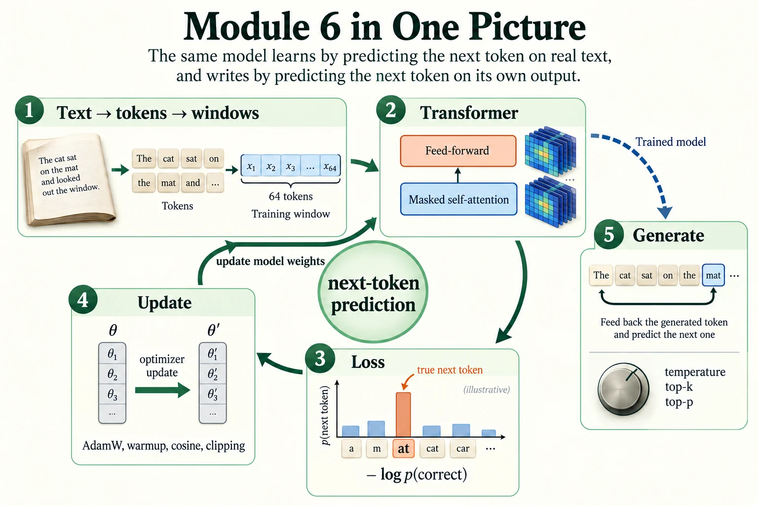
Figure 6.6.2. The training loop predicts real next tokens, measures loss and updates model weights. Generation branches from the trained model and feeds chosen tokens back into its context; it never runs the optimizer.
Summary
- Language models learn by next-token prediction, a self-supervised task: targets are the input shifted one position left.
- The loss is cross-entropy, −log(probability of the correct token), averaged over all positions. Read it against baselines (uniform, unigram, bigram).
- Teacher forcing feeds the true previous tokens during training, which makes all positions computable in parallel.
- Stable training uses AdamW, warmup, a cosine learning-rate schedule and gradient clipping; choose the learning rate on validation.
- Our model reached a validation loss of 1.742 (bigram 2.482), showed lower loss at positions with more short-range context, and learned "previous character" and "two characters back" attention heads.
- Generation is autoregressive: predict, choose, append, repeat.
- Greedy decoding repeated familiar words in this experiment; temperature trades correctness for variety; top-k and top-p remove unlikely tokens and balance the two.
- Inference needs no gradients, uses
model.eval(), runs one forward pass per new token (sped up by a KV cache), and suffers from exposure bias.
Glossary
| Term | Meaning |
|---|---|
| Next-token prediction | Predicting each token from the tokens before it. |
| Self-supervised learning | Learning from targets derived from the data itself. |
| Label shifting | Making targets by shifting the input one position left. |
| Cross-entropy loss | −log(probability of the correct token), averaged over positions. |
| Unigram / bigram baseline | A predictor using no context / only the previous token. |
| Teacher forcing | Training with the true previous tokens as input, not the model's own predictions. |
| AdamW | Adam with decoupled weight decay; the standard Transformer optimizer. |
| Weight decay | A small pull of weights towards zero, for regularisation. |
| Warmup | Increasing the learning rate gradually at the start of training. |
| Cosine decay | Lowering the learning rate along half a cosine wave. |
| Gradient clipping | Rescaling gradients whose norm exceeds a threshold. |
| Generalisation gap | The difference between training and validation loss. |
| Autoregressive generation | Producing tokens one at a time, each from the previous outputs. |
| Decoding strategy | The rule for choosing a token from the predicted distribution. |
| Greedy decoding | Always choosing the most likely token. |
| Temperature | A divisor of the logits that sharpens (< 1) or flattens (> 1) the distribution. |
| Top-k / top-p sampling | Sampling from the k most likely tokens / from the smallest set with total probability ≥ p. |
| KV cache | Stored keys and values of earlier tokens, reused during generation. |
| Exposure bias | The mismatch between training on real text and generating from the model's own output. |
Wrap-up
Quick check
What differs between the training and generation loops?
Training uses known histories and updates weights; generation chooses tokens from its evolving history.
What does gradient clipping at norm 1 do?
Rescale gradients only when their combined norm exceeds 1.
Why use both evaluation mode and no-grad inference?
Evaluation mode controls relevant layers; no-grad disables gradient tracking.
Questions and discussion
Ask about this lesson, share what you found in a lab, or help someone else. Posts are public on the course's GitHub Discussions: anyone can read them, and you need a GitHub account to post.
Opening it loads giscus from giscus.app.