From Sequences to Attention
Classroom material
- Time
- ~41 min
- Sections
- 9
- Code cells
- 18
- Labs
- 1
- Figures
- 8
Before you start
How can a network use the order of a sequence, and why did that lead to attention?
- You will be able to
- explain why order matters and why averaging loses it;
- describe how an RNN carries a hidden state from step to step, and compute one by hand;
- explain, with measurements, why RNNs struggle with long-range dependencies;
- explain how the LSTM's gates help, and when they do not help by default;
- explain the bottlenecks of sequential processing that attention removes.
At the end of Lesson 5.3 we found a model that could not understand "not good". It turned each word into a vector and averaged them, so it had no idea which word came first, or that "not" changes the word after it. The fault was not in the embeddings. It was in how the model combined them: averaging throws away order.
Language, music, speech, sensor readings, stock prices and DNA are all sequences: data where the order of the items carries meaning. This lesson is a short bridge between the embeddings of Lesson 5.3 and the Transformers of Module 6. We will see the first family of networks designed for sequences, the recurrent neural network (RNN), understand exactly where it struggles, and measure the problem for ourselves. Then we will see why the field moved to a different idea, attention, which is the heart of every modern language model.
This lesson is deliberately compact. RNNs are no longer the main tool for language, so the aim is not to master them but to understand the problems they faced, because those problems explain the design of the Transformer.
Key question: How can a network use the order of a sequence, and why did that lead to attention?
Prerequisites
read Lesson 5.3. You should be comfortable with embeddings, the training loop, and the idea of a gradient flowing backwards through a network.
Setup — imports, versions and device detection used by the notebook (1 cells)
Run this cell first. This lesson uses no dataset: every experiment uses small, randomly generated sequences, so you can see each effect in isolation. All the experiments together run in about a minute on a CPU.
Environment and results. The saved outputs record one CPU reference run; random seeds reduce variation but do not guarantee identical numbers across computers. Read the comparisons as evidence from that run. Training times depend on your hardware.
If packages are missing, install them into your notebook environment, then restart the kernel and run from the beginning:
%pip install torch==2.14.1 numpy==2.5.4 pandas==3.0.6 matplotlib==3.11.2 scikit-learn==1.9.1 scipy==1.18.1
import collectionsimport numpy as npimport torchimport torch.nn as nnimport torch.nn.functional as Fimport matplotlib.pyplot as plttorch.manual_seed(0)np.random.seed(0)print("PyTorch", torch.__version__)PyTorch 2.14.1+cu130
Why Sequence Order Matters
Consider two sentences: "dog bites man" and "man bites dog". They contain exactly the same words, but one is ordinary and the other is news. Any representation that treats a sentence as a bag of words, simply counting which words occur, cannot tell them apart:
a, b = "dog bites man".split(), "man bites dog".split()print("bag of words, sentence A:", sorted(collections.Counter(a).items()))print("bag of words, sentence B:", sorted(collections.Counter(b).items()))print("identical bags?", collections.Counter(a) == collections.Counter(b))bag of words, sentence A: [('bites', 1), ('dog', 1), ('man', 1)]
bag of words, sentence B: [('bites', 1), ('dog', 1), ('man', 1)]
identical bags? True
The two bags are identical. And if we average the embedding vectors of the words, as our sentiment model did in Lesson 5.3, the result is also identical, whatever the embeddings are:
torch.manual_seed(0)vocab = {"dog": 0, "bites": 1, "man": 2}emb = nn.Embedding(3, 4)ea, eb = emb(torch.tensor([vocab[w] for w in a])), emb(torch.tensor([vocab[w] for w in b]))print("cosine of averaged embeddings:", round(F.cosine_similarity(ea.mean(0), eb.mean(0), dim=0).item(), 4))cosine of averaged embeddings: 1.0
A cosine similarity of 1.0 means the two sentences get exactly the same representation. Averaging is order-blind: adding up the same vectors in a different order always gives the same total.
The same problem appears everywhere in sequences. "Not good" and "good, not" mean different things. In a sensor reading, a temperature that rises then falls is different from one that falls then rises. What we need is a way of combining a sequence that depends on the order of its items.
Key terms
- Sequence: an ordered list of items, such as words in a sentence or readings over time.
- Bag of words: a representation that records which words appear (and how often) but not their order.
- Order-blind: giving the same result whatever order the inputs come in.
-
Name one other everyday example (not language) where two sequences contain the same items but mean different things because of their order.
Many answers work. For example: the steps of a recipe (mix then bake is not the same as bake then mix), a phone number or PIN, a sequence of moves in a game, or a patient's symptoms appearing in a particular order.
Why do averaged word embeddings fail on reversed word order?
Averaging the same vectors gives the same result regardless of order.
Recurrent Neural Networks: The Complete Picture
Think about how you read this sentence. You don't hold every previous word separately in mind. You keep a running sense of "what this is about so far", and update it as each new word arrives.
A recurrent neural network (RNN) does exactly that. It reads a sequence one item at a time, in order, and keeps a vector called the hidden state, its running memory. At each step it combines two things: the new input and its previous hidden state. Its output is a new hidden state, which is carried forward to the next step.
The update rule at each step t is:
where:
- x_t is the input at step t (for example, the embedding of word t);
- h_(t−1) is the hidden state from the previous step (it starts as all zeros);
- W_x and W_h are weight matrices, and b is a bias; the same weights are used at every step;
- tanh (the hyperbolic tangent) squashes each value into the range −1 to +1, so the hidden state cannot grow without limit.
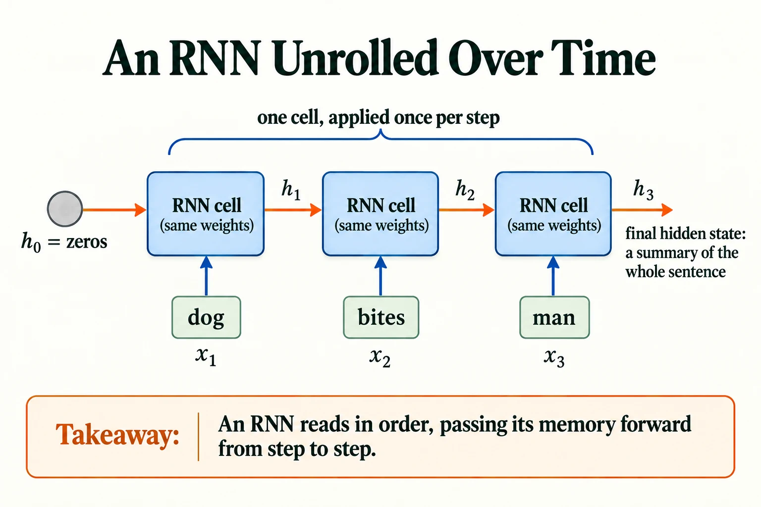
Figure 5.4.1. One recurrent update with shared weights reads dog → bites → man. Each hidden state depends on the current token and previous state; the final state is a finite-dimensional sequence summary.
The second term, W_h h_(t−1), is what makes the network recurrent: the output of the network feeds back into itself. Let's write this loop by hand, with tiny sizes so that every number is visible: 4 numbers per input word and 3 numbers in the hidden state.
torch.manual_seed(0)D_IN, D_H = 4, 3W_x = torch.randn(D_H, D_IN) * 0.5 # input -> hiddenW_h = torch.randn(D_H, D_H) * 0.5 # hidden -> hidden (the "memory" connection)bias = torch.zeros(D_H)def rnn_by_hand(xs): """Apply the shared RNN update in temporal order and return every hidden state. Arguments: xs: Input-vector sequence in temporal order. """ h = torch.zeros(D_H) # the memory starts empty states = [] for x_t in xs: # one step per token, in order h = torch.tanh(W_x @ x_t + W_h @ h + bias) states.append(h) return torch.stack(states)with torch.no_grad(): hs = rnn_by_hand(ea)for word, h in zip(a, hs): print(f"after '{word}':", [round(v, 3) for v in h.tolist()])after 'dog': [0.999, -0.681, 0.204] after 'bites': [-0.941, 0.98, 0.626] after 'man': [0.672, 0.388, 0.319]
After reading "dog", the hidden state is [0.999, −0.681, 0.204]. After "bites" it has changed to [−0.941, 0.98, 0.626], and after "man" to [0.672, 0.388, 0.319]. Every value stays between −1 and +1, because of tanh. The final hidden state is the network's summary of the whole sentence.
PyTorch provides the same thing as nn.RNN. If we copy our weights into it, it should give identical results:
rnn = nn.RNN(input_size=D_IN, hidden_size=D_H, batch_first=True)with torch.no_grad(): rnn.weight_ih_l0.copy_(W_x); rnn.weight_hh_l0.copy_(W_h) rnn.bias_ih_l0.zero_(); rnn.bias_hh_l0.zero_() out, h_last = rnn(ea.unsqueeze(0)) # input (batch=1, T=3, 4)print("output (all hidden states):", tuple(out.shape), "| final hidden state:", tuple(h_last.shape))print("matches our loop?", torch.allclose(out[0], hs, atol=1e-6))output (all hidden states): (1, 3, 3) | final hidden state: (1, 1, 3) matches our loop? True
It matches. Note the two outputs of nn.RNN: out holds the hidden state at every step, shape (batch, T, hidden) = (1, 3, 3), and h_last holds only the final hidden state, shape (layers, batch, hidden) = (1, 1, 3). With batch_first=True, PyTorch expects inputs as (batch, T, features).
Common mistake: forgetting
batch_first=True. Without it, PyTorch's recurrent layers expect(T, batch, features), and will silently treat your batch dimension as time if the shapes happen to fit.
Now the key test. Does the RNN tell "dog bites man" from "man bites dog"?
with torch.no_grad(): h_a, h_b = rnn_by_hand(ea)[-1], rnn_by_hand(eb)[-1]print("final state, 'dog bites man':", [round(v, 3) for v in h_a.tolist()])print("final state, 'man bites dog':", [round(v, 3) for v in h_b.tolist()])print("cosine of final states:", round(F.cosine_similarity(h_a, h_b, dim=0).item(), 4))final state, 'dog bites man': [0.672, 0.388, 0.319] final state, 'man bites dog': [1.0, -0.804, -0.164] cosine of final states: 0.2831
Yes. The final states are very different, with a cosine similarity of only 0.2831, compared with 1.0 for averaging. Because each step depends on everything before it, the same words in a different order produce a different memory. The RNN is order-aware.
Key terms
- Recurrent neural network (RNN): a network that processes a sequence one step at a time, carrying a hidden state forward.
- Hidden state: the RNN's running memory; a vector updated at every step.
- Unrolling: drawing (or computing) an RNN as one copy of the cell per step, connected by the hidden state.
-
An RNN has a hidden state of 32 numbers. How many numbers does it carry forward after reading a sequence of 5 words? After 5,000 words?
32 numbers in both cases. The hidden state has a fixed size, whatever the length of the sequence. That is the information bottleneck of Section 5.
What changes from one RNN step to the next?
The hidden state; the update weights are shared.
Why Standard RNNs Struggle with Long-Term Dependencies
Order-awareness is a good start. But consider this sentence:
"The film, which was shot over three years in four countries with a cast of hundreds and a famously difficult director, was a triumph."
To know that "was" (singular) is correct, the network must connect it to "film", many words earlier. A connection like this, between items far apart in a sequence, is a long-term dependency. Can an RNN learn one?
3.1 Measuring how far the gradient reaches
The RNN learns, like every network, through backpropagation. Recall from Module 1 that backpropagation is credit assignment: it works out how much each input and weight contributed to the error. For an RNN, the gradient has to travel backwards through every step, from the final output back to the early inputs. Let's measure how much of it arrives.
We feed a random sequence of 60 inputs into an untrained RNN, take its final output, and backpropagate. The size of the gradient at each input position tells us how strongly the final output depends on that input, and so how much that input can be "learned from". We average over 3 random starting weights.
def gradient_reach(make_model, T=60, seeds=(0, 1, 2)): """Average input-gradient norms across initialisation seeds, indexed by distance back from the last output. Arguments: make_model: Factory creating a fresh model for each probe seed. T: Sequence length, or text-vector batch in contrastive_loss. seeds: Initialisation seeds to average over. """ curves = [] for s in seeds: torch.manual_seed(s) model = make_model() x = torch.randn(1, T, 16, requires_grad=True) out = model(x) # (1, T, hidden) out[0, -1].sum().backward() # how much does the final output depend on each input? curves.append(x.grad[0].norm(dim=1)) # (T,) one number per position g = torch.stack(curves).mean(0) return g.flip(0) # index k = k steps back from the endclass RNNWrap(nn.Module): """Expose a recurrent layer's sequence output through the shared probe interface.""" def __init__(self, cell): """Create the components of this model; the forward computation is traced in the lesson. Arguments: cell: The recurrent PyTorch layer whose sequence outputs are exposed. """ super().__init__(); self.cell = cell def forward(self, x): """Expose a recurrent layer's sequence output through the shared probe interface. Arguments: x: Floating-point tensor; image models use (B, C, H, W), token-vector models use (B, T, D). """ return self.cell(x)[0]make_rnn = lambda: RNNWrap(nn.RNN(16, 32, batch_first=True))g_rnn = gradient_reach(make_rnn)for k in [0, 1, 5, 10, 20, 40]: print(f"{k:>2} steps back: gradient size {g_rnn[k].item():.1e}")0 steps back: gradient size 1.9e+00 1 steps back: gradient size 1.0e+00 5 steps back: gradient size 5.5e-02 10 steps back: gradient size 2.9e-03 20 steps back: gradient size 2.3e-06 40 steps back: gradient size 8.8e-12
The gradient shrinks dramatically with distance: about 1.9 for the very last input, 0.055 five steps back, 0.0029 ten steps back, 0.0000023 twenty steps back, and 8.8e-12 forty steps back. (The notation 8.8e-12 means 8.8 × 10⁻¹², a decimal point followed by eleven zeros and then 88.) For practical purposes, an input 40 steps back has no influence on learning at all. This is the vanishing gradient problem, which you met in Module 3. In an RNN it is especially severe, because the "depth" of the network is the length of the sequence.
3.2 Why it vanishes: repeated multiplication
Every step backwards multiplies the gradient by the same kind of factor: the recurrent weights W_h, times the slope of tanh. If that factor is a little less than 1, repeating it many times drives the result towards zero; if it is a little more than 1, the result explodes.
print("0.9 multiplied by itself 40 times:", f"{0.9 ** 40:.4f}")print("0.5 multiplied by itself 40 times:", f"{0.5 ** 40:.1e}")print("1.1 multiplied by itself 40 times:", f"{1.1 ** 40:.1f}")z = torch.linspace(-4, 4, 9)print("slope of tanh at", z.tolist(), ":\n", [round(v, 3) for v in (1 - torch.tanh(z) ** 2).tolist()])0.9 multiplied by itself 40 times: 0.0148 0.5 multiplied by itself 40 times: 9.1e-13 1.1 multiplied by itself 40 times: 45.3 slope of tanh at [-4.0, -3.0, -2.0, -1.0, 0.0, 1.0, 2.0, 3.0, 4.0] : [0.001, 0.01, 0.071, 0.42, 1.0, 0.42, 0.071, 0.01, 0.001]
Multiplying by 0.9 forty times leaves 0.0148; multiplying by 0.5 forty times leaves 9.1e-13, essentially nothing. Multiplying by 1.1 forty times gives 45.3: the opposite problem, an exploding gradient. A factor of exactly 1 at every step is almost impossible to maintain.
The tanh function makes vanishing more likely. Its slope is 1.0 at zero but drops quickly away from zero: 0.42 at ±1, 0.071 at ±2 and 0.01 at ±3. So whenever the hidden state is pushed towards ±1, which tanh does to large values, the gradient flowing back through that step is multiplied by a small number. Here is the measurement from Section 3.1 as a plot. On a logarithmic scale, a constant shrinking factor per step shows up as a straight downward line.
plt.figure(figsize=(6.5, 3.8))plt.semilogy(g_rnn.numpy(), label="vanilla RNN")plt.xlabel("how many steps back the input was"); plt.ylabel("gradient size (log scale)")plt.title("How much the last output 'feels' each earlier input"); plt.grid(alpha=0.3); plt.legend()plt.tight_layout(); plt.show()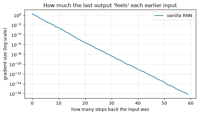
3.3 Does it matter in practice? A memory test
A vanishing gradient is a warning sign, but the real question is whether the network can still learn a long-range task. So let's set it one. Each sequence is a list of random tokens. The first token is a clue, 0 or 1, and the label is simply that clue. Everything after it is noise. To succeed, the network must remember the first token all the way to the end, and it classifies using only its final hidden state. By changing the sequence length, we control exactly how far the information has to travel.
def make_task(n, T, seed): """Generate random sequences whose binary label is encoded only in the first token. Arguments: n: Number of synthetic examples. T: Sequence length, or text-vector batch in contrastive_loss. seed: Random seed for this experiment. """ g = torch.Generator().manual_seed(seed) x = torch.randint(2, 10, (n, T), generator=g) y = torch.randint(0, 2, (n,), generator=g) x[:, 0] = y return x, yprint(make_task(2, 10, seed=0))class SeqClassifier(nn.Module): """Embed a sequence and classify from its final recurrent hidden state.""" def __init__(self, kind="rnn", forget_bias=None): """Create the components of this model; the forward computation is traced in the lesson. Arguments: kind: The model or mask family selected in the surrounding example. forget_bias: Optional value assigned to each of the two LSTM forget-gate bias slices. """ super().__init__() self.emb = nn.Embedding(10, 16) self.rnn = (nn.RNN if kind == "rnn" else nn.LSTM)(16, 32, batch_first=True) if forget_bias is not None: # LSTM only: start with the forget gate open (see Section 4) with torch.no_grad(): for b_ in [self.rnn.bias_ih_l0, self.rnn.bias_hh_l0]: b_[32:64] = forget_bias self.out = nn.Linear(32, 2) def forward(self, x): """Embed a sequence and classify from its final recurrent hidden state. Arguments: x: Integer token-ID batch shaped (B, T). """ h, _ = self.rnn(self.emb(x)) # (B, T, 32) return self.out(h[:, -1]) # classify from the LAST hidden state onlydef run_task(T, seed, **kw): """Train and validate a fresh recurrent classifier on the controlled first-token memory task. Arguments: T: Sequence length, or text-vector batch in contrastive_loss. seed: Random seed for this experiment. **kw: Recurrent-classifier options forwarded to SeqClassifier. """ Xt, yt = make_task(4000, T, seed=100) # training sequences Xv, yv = make_task(1000, T, seed=200) # validation sequences torch.manual_seed(seed) m = SeqClassifier(**kw); opt = torch.optim.Adam(m.parameters(), lr=3e-3) for epoch in range(8): perm = torch.randperm(len(Xt)) for i in range(0, len(Xt), 64): b_ = perm[i:i+64] opt.zero_grad(); F.cross_entropy(m(Xt[b_]), yt[b_]).backward(); opt.step() with torch.no_grad(): return (m(Xv).argmax(1) == yv).float().mean().item()(tensor([[0, 9, 7, 2, 5, 5, 5, 9, 3, 5],
[1, 4, 6, 9, 8, 2, 2, 6, 4, 3]]), tensor([0, 1]))
The two example sequences start with 0 and 1, and their labels are 0 and 1. Now we train an RNN at four lengths, with 3 different random seeds each, and measure accuracy on 1,000 validation sequences. Guessing would score about 0.5, and each validation sequence is worth 0.001 of accuracy.
LENGTHS, SEEDS = [10, 30, 50, 100], [0, 1, 2]task_results = {}for T in LENGTHS: accs = [run_task(T, s, kind="rnn") for s in SEEDS] task_results[("RNN", T)] = accs print(f"vanilla RNN, length {T:>3}: val acc per seed {[round(a_, 3) for a_ in accs]}")print("one validation sequence is worth", 1 / 1000, "of accuracy; guessing gives about 0.5")vanilla RNN, length 10: val acc per seed [1.0, 1.0, 1.0] vanilla RNN, length 30: val acc per seed [0.475, 0.461, 1.0] vanilla RNN, length 50: val acc per seed [0.511, 0.494, 0.51] vanilla RNN, length 100: val acc per seed [0.533, 0.518, 0.501] one validation sequence is worth 0.001 of accuracy; guessing gives about 0.5
At length 10, every seed solves the task perfectly (1.0). At length 30, only one of the three seeds succeeds; the other two score 0.475 and 0.461, no better than guessing. At lengths 50 and 100, every seed fails, with accuracies between 0.494 and 0.533.
The task itself is trivial: "repeat the first token". The RNN fails not because the task is hard, but because the error signal from the end of the sequence cannot reach the first step to teach it what to remember. This is the long-term-dependency problem, measured directly.
Key terms
- Long-term dependency: a relationship between items far apart in a sequence.
- Vanishing gradient: a gradient that shrinks towards zero as it travels back through many steps, so early inputs cannot be learned from.
- Exploding gradient: a gradient that grows uncontrollably as it travels back.
-
Why does the RNN succeed at length 10 but fail at length 50, when the rule to learn ("output the first token") is exactly the same?
The rule is the same, but the distance the learning signal must travel is not. At length 50, the gradient from the final output must pass back through 49 steps before reaching the first token, and it shrinks at every step, so almost nothing arrives to teach the network what it should have stored. At length 10, enough of the gradient survives.
Why is a long-range memory task harder for a basic RNN?
The learning signal passes through many recurrent transformations.
LSTM and GRU: The Intuition Behind Gating Mechanisms (Extension)
This section goes a little deeper than the rest of the note. The key idea, that gates let a network choose what to keep, is worth understanding; the details are optional.
The vanilla RNN overwrites its entire memory at every step: the new hidden state is a fresh tanh of a mix of input and old memory. The Long Short-Term Memory (LSTM) network, designed specifically to solve the problem we just measured, changes this. It keeps a separate memory, the cell state, and controls it with gates.
A gate is a set of numbers between 0 and 1, produced by a sigmoid function, that is multiplied element by element with some other vector. A gate value of 1 lets everything through; 0 blocks everything. The LSTM has three:
- the forget gate decides how much of the old cell state to keep;
- the input gate decides how much new information to write;
- the output gate decides how much of the cell state to reveal as the hidden state.
The crucial change is in how memory is carried forward. Instead of being squashed through tanh at every step, the cell state is updated mostly by multiplying by the forget gate and adding new information. If the forget gate stays close to 1, the memory, and the gradient flowing back along it, passes from step to step almost unchanged.
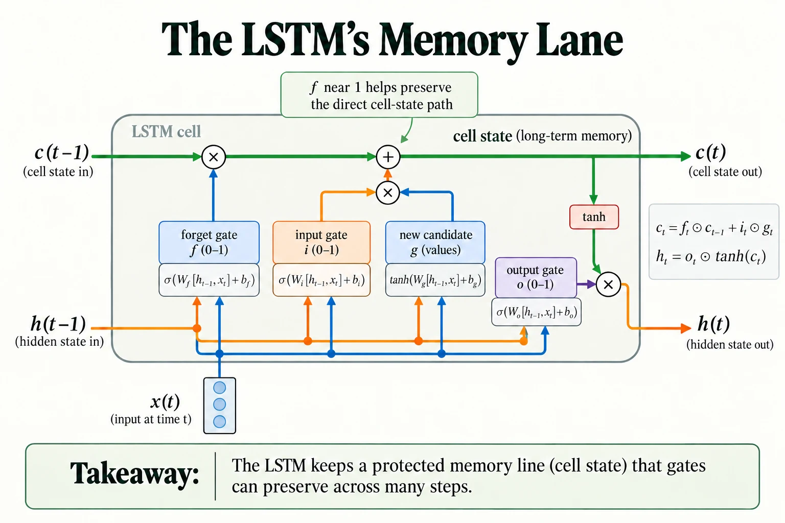
Figure 5.4.2. The forget gate retains old cell state, the input gate admits a candidate, and the output gate exposes tanh of the new state. A near-one forget gate helps preserve the direct memory path; it does not guarantee perfect long-range learning.
4.1 The catch: the gate must start open
Here is a detail that is easy to miss. The forget gate is computed with a sigmoid of a weighted sum plus a bias. PyTorch starts all biases at around zero, so at the start of training the forget gate sits at about sigmoid(0):
sig = torch.sigmoidprint(f"forget gate at the start of training (bias 0): sigmoid(0) = {sig(torch.tensor(0.)).item():.3f}")print(f"forget gate with bias 1.5 + 1.5 = 3: sigmoid(3) = {sig(torch.tensor(3.)).item():.3f}")print(f"memory kept after 40 steps at 0.5 per step: {0.5 ** 40:.1e}")print(f"memory kept after 40 steps at 0.953 per step: {sig(torch.tensor(3.)).item() ** 40:.3f}")forget gate at the start of training (bias 0): sigmoid(0) = 0.500 forget gate with bias 1.5 + 1.5 = 3: sigmoid(3) = 0.953 memory kept after 40 steps at 0.5 per step: 9.1e-13 memory kept after 40 steps at 0.953 per step: 0.143
In this zero-logit illustration, the forget gate is 0.500, retaining half the old cell state per step along this direct path. Actual gates vary with the inputs, previous state, random weights and biases; PyTorch does not fix them all at exactly 0.5. After 40 steps that leaves 9.1e-13, the same vanishing as a plain RNN. If instead we set the forget-gate bias so that the gate starts at sigmoid(3) = 0.953, the memory kept after 40 steps is 0.143, enormously more. (Each LSTM has two bias vectors that are added together, so setting each to 1.5 gives a total of 3.) Starting the forget gate open is a well-known practical technique.
Let's test both versions of the LSTM on the same memory task.
for name, kw in [("LSTM (default start)", dict(kind="lstm")), ("LSTM (forget gate open)", dict(kind="lstm", forget_bias=1.5))]: for T in LENGTHS: accs = [run_task(T, s, **kw) for s in SEEDS] task_results[(name, T)] = accs print(f"{name:<24} length {T:>3}: val acc per seed {[round(a_, 3) for a_ in accs]}")LSTM (default start) length 10: val acc per seed [1.0, 1.0, 1.0] LSTM (default start) length 30: val acc per seed [0.502, 0.495, 0.471] LSTM (default start) length 50: val acc per seed [0.506, 0.511, 0.505] LSTM (default start) length 100: val acc per seed [0.523, 0.506, 0.528] LSTM (forget gate open) length 10: val acc per seed [1.0, 1.0, 1.0] LSTM (forget gate open) length 30: val acc per seed [1.0, 1.0, 1.0] LSTM (forget gate open) length 50: val acc per seed [1.0, 1.0, 1.0] LSTM (forget gate open) length 100: val acc per seed [1.0, 1.0, 1.0]
The results are striking:
- The default LSTM does no better than the vanilla RNN. It solves length 10, but fails at length 30 on all three seeds (0.471 to 0.502), and at every longer length.
- The LSTM with its forget gate open scores 1.0 on every seed, at every length, all the way to 100.
The plot shows all three models; each line is the average over seeds, and the faint dots are individual seeds.
fig, ax = plt.subplots(figsize=(6.5, 3.8))for (name, marker) in [("RNN", "o"), ("LSTM (default start)", "s"), ("LSTM (forget gate open)", "^")]: means = [np.mean(task_results[(name, T)]) for T in LENGTHS] ax.plot(LENGTHS, means, marker=marker, label=name) for T in LENGTHS: ax.scatter([T] * len(SEEDS), task_results[(name, T)], marker=marker, alpha=0.3, color=ax.lines[-1].get_color())ax.axhline(0.5, color="grey", ls="--", lw=1, label="guessing")ax.set_xlabel("sequence length (distance from the clue to the answer)"); ax.set_ylabel("validation accuracy")ax.set_title("Remembering the first token (line = mean, faint dots = individual seeds)")ax.set_ylim(0.4, 1.05); ax.grid(alpha=0.3); ax.legend(fontsize=8); plt.tight_layout(); plt.show()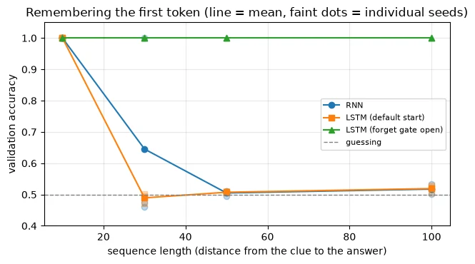
The gradient measurement from Section 3.1 tells the same story from the inside:
def open_lstm(): """Create an LSTM with both forget-gate bias slices set to 1.5, then wrap its sequence output.""" lstm = nn.LSTM(16, 32, batch_first=True) with torch.no_grad(): for b_ in [lstm.bias_ih_l0, lstm.bias_hh_l0]: b_[32:64] = 1.5 return RNNWrap(lstm)g_lstm = gradient_reach(lambda: RNNWrap(nn.LSTM(16, 32, batch_first=True)))g_open = gradient_reach(open_lstm)for k in [10, 20, 40]: print(f"{k:>2} steps back: RNN {g_rnn[k].item():.1e} | LSTM {g_lstm[k].item():.1e} | LSTM open {g_open[k].item():.1e}")10 steps back: RNN 2.9e-03 | LSTM 5.0e-03 | LSTM open 1.8e-01 20 steps back: RNN 2.3e-06 | LSTM 5.4e-05 | LSTM open 2.1e-01 40 steps back: RNN 8.8e-12 | LSTM 6.1e-09 | LSTM open 3.0e-01
Forty steps back, the gradient is 8.8e-12 for the RNN, 6.1e-09 for the default LSTM, and 0.30 for the open-gate LSTM. The open forget gate keeps the gradient path alive.
So the honest summary is: gates make long-term memory possible, but they have to be used that way. An LSTM's architecture allows memory to persist; whether it does depends on the gate values, which are learned, and which need a good starting point.
The Gated Recurrent Unit (GRU) is a simplified relative of the LSTM. It merges the cell state and hidden state and uses two gates instead of three, so it is a little cheaper. With an input size of 16 and a hidden size of 32, a vanilla RNN has 1,600 parameters, a GRU 4,800 and an LSTM 6,400: each gate needs its own weights.
print("parameters with input 16 and hidden 32:")for name, cell in [("RNN", nn.RNN(16, 32)), ("GRU", nn.GRU(16, 32)), ("LSTM", nn.LSTM(16, 32))]: print(f" {name:<5} {sum(p.numel() for p in cell.parameters()):>5}")parameters with input 16 and hidden 32: RNN 1600 GRU 4800 LSTM 6400
Key terms
- LSTM (Long Short-Term Memory): a recurrent network with a protected cell state controlled by forget, input and output gates.
- GRU (Gated Recurrent Unit): a simpler gated recurrent network with two gates.
- Gate: a vector of values between 0 and 1 (from a sigmoid) that scales another vector, letting information through or blocking it.
- Cell state: the LSTM's long-term memory line.
-
The default LSTM failed the length-30 task even though its architecture is designed for long memory. In one sentence, why?
Its forget gate started at about 0.5, so it kept only half its memory per step, and the memory (and gradient) vanished almost as fast as in a plain RNN, before the gates could learn to stay open.
Visual walkthrough: Inspect one LSTM memory update.
Follow one scalar coordinate through the forget, input and output gates. The values are a worked example.
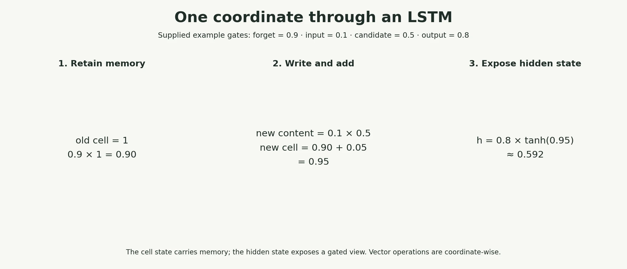
These supplied numbers illustrate the calculation. The web app adds a paused, step-by-step animation of the same example.
Paused on arrival. Use Previous step, Play/Pause, Next step or Reset. This is a fixed worked example, not a live trained model.
What makes an LSTM's memory path useful?
Learned gates can preserve cell-state information across steps.
The Limitations of Recurrent Processing
If an LSTM with a well-set forget gate can carry a fact across 100 steps, why did the field move on? Because remembering one fact is not the only requirement. Real language tasks expose two deeper limitations that no choice of gates can remove.
Limitation 1: everything must squeeze through one fixed-size memory. However long the sequence is, the RNN carries forward only its hidden state.
torch.manual_seed(0)cell = nn.RNN(16, 32, batch_first=True)for T in [10, 1000]: out, h_final = cell(torch.randn(1, T, 16)) print(f"T={T:>4}: everything the RNN carries forward is h_final {tuple(h_final.shape)}") print(f" steps that must run one after another: {T}")X = torch.randn(1000, 32)scores = X @ X.T # every position compared with every other, in ONE matrix multiplicationprint("all pairwise scores for 1000 positions:", tuple(scores.shape), "computed in a single operation")T= 10: everything the RNN carries forward is h_final (1, 1, 32)
steps that must run one after another: 10
T=1000: everything the RNN carries forward is h_final (1, 1, 32)
steps that must run one after another: 1000
all pairwise scores for 1000 positions: (1000, 1000) computed in a single operation
With a hidden size of 32, the RNN carries forward a (1, 1, 32) state after 10 steps, and exactly the same 32 numbers after 1,000 steps. Every fact from a 1,000-word document (names, dates, who did what to whom) must be compressed into those 32 numbers before the end. Adding facts means overwriting others. This is called the information bottleneck.
Limitation 2: the steps must run one after another. To compute the hidden state at step 1,000, the RNN needs the state at step 999, which needs step 998, and so on: 1,000 steps that cannot be done at the same time. Modern hardware such as GPUs is fast precisely because it does thousands of calculations in parallel. A sequential loop wastes most of that power, which makes RNNs slow to train on large datasets.
Compare the last line of the output. Comparing every position with every other position, for all 1,000 positions, is a single matrix multiplication producing a (1000, 1000) grid of scores. All of it can be computed at once. That operation is the core of attention.
Which limitation remains even with good recurrent memory?
Hidden states still depend on sequential computation.
From Sequential Processing to Attention
Attention takes a completely different approach. Instead of passing information along a chain, step by step, it lets each position look directly at every other position and decide how much to take from each one.
Here is the idea in one picture. To build its representation, the last word in a sentence asks a question, its query. Every word in the sentence offers a key, a description of what it contains, and a value, the information it can contribute. The query is compared with every key to produce a score; the scores are turned into weights that sum to 1 (with softmax); and the result is a weighted average of the values. A word that is relevant to the query gets a large weight, however far away it is.
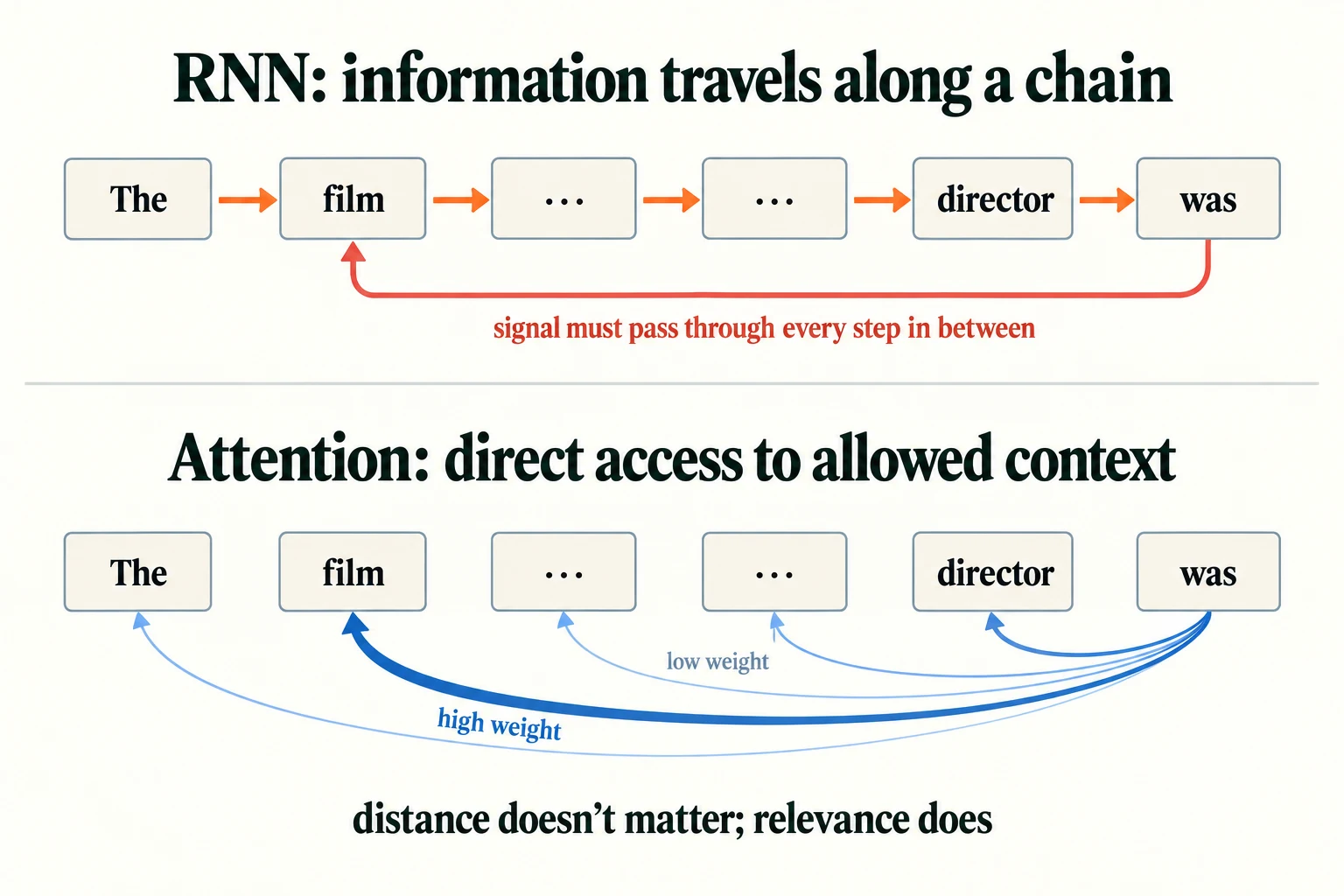
Figure 5.4.3. Recurrent information follows sequential updates; attention can directly mix allowed context positions. Connection strengths are illustrative. A causal model can consult only the current and earlier positions.
Let's build the smallest possible version of this, a single attention step in which the last position attends to all 60 positions, and run the same gradient measurement as in Section 3.1. We will study queries, keys and values properly in Module 6; for now, watch what happens to the gradient.
class TinyAttention(nn.Module): """Let the last input position attend directly to all input positions for the gradient probe.""" def __init__(self, d=16, h=32): """Create the components of this model; the forward computation is traced in the lesson. Arguments: d: Input vector width (or sinusoidal feature width in sinusoidal). h: Projected attention width. """ super().__init__() self.q, self.k, self.v = nn.Linear(d, h), nn.Linear(d, h), nn.Linear(d, h) def forward(self, x): # x: (1, T, d) """Let the last input position attend directly to all input positions for the gradient probe. Arguments: x: Floating-point tensor; image models use (B, C, H, W), token-vector models use (B, T, D). """ q = self.q(x[:, -1:]) # (1, 1, h) a "question" from the last position k, v = self.k(x), self.v(x) # (1, T, h) each position's "label" and "content" w = torch.softmax(q @ k.transpose(1, 2) / k.shape[-1] ** 0.5, dim=-1) # (1, 1, T) weights sum to 1 self.weights = w.detach() out = w @ v # (1, 1, h) weighted average of contents return out.expand(-1, x.shape[1], -1) # same shape as an RNN's output, for comparisong_att = gradient_reach(TinyAttention)for k in [0, 10, 20, 40, 59]: print(f"{k:>2} steps back: attention {g_att[k].item():.1e} | RNN {g_rnn[k].item():.1e}")0 steps back: attention 2.4e-01 | RNN 1.9e+00 10 steps back: attention 5.2e-02 | RNN 2.9e-03 20 steps back: attention 5.4e-02 | RNN 2.3e-06 40 steps back: attention 4.0e-02 | RNN 8.8e-12 59 steps back: attention 3.9e-02 | RNN 7.3e-17
Through attention, the gradient reaching an input 59 steps back is 3.9e-02, about the same as for an input 10 steps back (5.2e-02). Through the RNN, the input 59 steps back receives 7.3e-17. The most recent position gets a larger gradient under attention (2.4e-01) only because it also supplies the query. Here are all four measurements together:
plt.figure(figsize=(7, 4))for g, lab in [(g_rnn, "vanilla RNN"), (g_lstm, "LSTM (default start)"), (g_open, "LSTM (forget gate open)"), (g_att, "attention")]: plt.semilogy(g.numpy(), label=lab)plt.xlabel("how many steps back the input was"); plt.ylabel("gradient size (log scale)")plt.title("Gradient reaching each earlier input from the last output (average of 3 seeds)")plt.grid(alpha=0.3); plt.legend(); plt.tight_layout(); plt.show()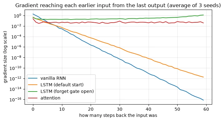
The picture summarises this whole note:
- The vanilla RNN (blue) and default LSTM (orange) fall in straight lines: their gradients shrink by a constant factor per step.
- The open-gate LSTM (green) keeps its gradient, and even grows slightly towards the far past, but it still has the fixed-size bottleneck and still has to process one step at a time.
- Attention (red) is flat: every input is one step away from the output, so distance simply does not matter.
Attention solves all three problems at once:
- No long chain: every position connects directly to every other, so gradients do not have to survive many multiplications.
- No single bottleneck: each position keeps its own vector, and any position can draw on any other, so information does not all have to fit into one hidden state.
- Parallel computation: all the comparisons are matrix multiplications that run at once on a GPU.
It also gives us what Lesson 5.3 was missing: contextual representations. When "bank" attends to "river", or "good" attends to "not", its new vector reflects its surroundings.
Attention has a price. Comparing every position with every other means the number of comparisons grows with the square of the sequence length. For 1,000 positions, that was a (1000, 1000) grid, a million scores. You will meet this cost, and how it is managed, in Module 6.
Common mistake: concluding that RNNs "cannot remember". As you measured, a well-initialised LSTM carried a fact across 100 steps perfectly. The reasons attention replaced recurrence for language are the fixed-size bottleneck and sequential computation, together with attention's direct access to every position.
Key terms
- Attention: a mechanism in which each position computes a weighted average of other positions' information, with weights based on relevance.
- Query, key, value: what a position is looking for, what each position offers as a description, and the information each position contributes.
- Information bottleneck: forcing all information through a fixed-size representation.
- Parallel computation: performing many calculations at the same time instead of one after another.
-
Give two reasons, other than vanishing gradients, why processing a 10,000-word document with an RNN is difficult.
First, everything must be compressed into a fixed-size hidden state, so facts from early in the document are overwritten by later ones (the information bottleneck). Second, the 10,000 steps must be computed one after another, which makes training slow and wastes the parallel power of modern hardware.
What does attention provide to a distant token?
A direct weighted path to relevant values, subject to the mask.
Putting It All Together
Sequences carry meaning in their order, but a bag of words, or an average of embeddings, is order-blind: "dog bites man" and "man bites dog" got identical representations (cosine 1.0).
An RNN reads one item at a time and carries a hidden state forward, so order changes its memory (final-state cosine 0.2831). But to learn, its gradient must travel back through every step, and it is multiplied by a shrinking factor each time. Forty steps back, it had fallen to 8.8e-12. On a task as simple as "remember the first token", the RNN succeeded at length 10 and failed beyond 30.
The LSTM adds a protected cell state controlled by gates. With its forget gate starting open, it solved the task at every length up to 100, and its gradient no longer vanished (0.30 forty steps back). With the default start, it failed just like the RNN. Gates make long memory possible; they do not guarantee it.
Even a good LSTM keeps two limitations: all information must pass through a fixed-size hidden state, 32 numbers whether the sequence has 10 steps or 1,000, and the steps must run one after another. Attention removes both. Each position looks directly at every other position and takes a relevance-weighted average, all in parallel. Its gradient reach was flat across all 60 positions. That idea, developed fully, is the Transformer, the subject of Module 6.
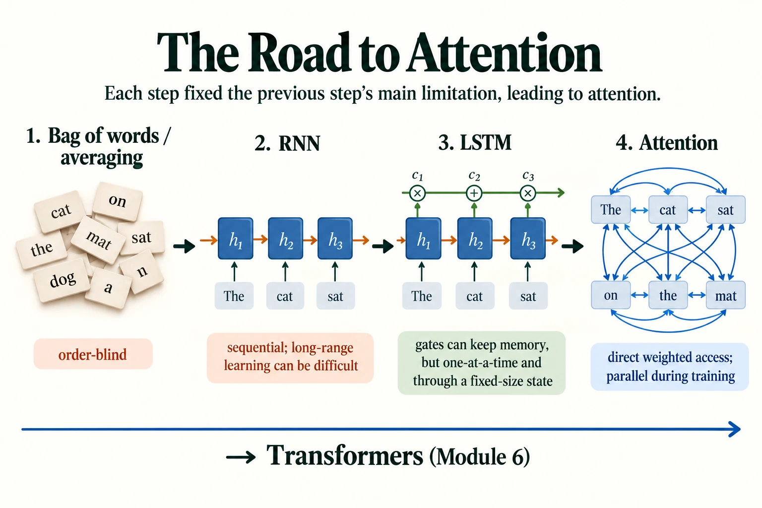
Figure 5.4.4. Order-aware recurrence, gated memory and direct attention address different limitations. Attention supports parallel training, while autoregressive generation still proceeds one new token at a time.
Summary
- In sequences, order carries meaning. Bags of words and averaged embeddings are order-blind.
- An RNN processes one item at a time with the rule h_t = tanh(W_x x_t + W_h h_(t−1) + b), using the same weights at every step and carrying a hidden state forward. It is order-aware.
- Backpropagating through many steps multiplies the gradient by similar factors repeatedly, so it vanishes (or explodes). We measured it falling to 8.8e-12 forty steps back.
- On a "remember the first token" task, a vanilla RNN failed beyond length 30, even though the rule never changed.
- LSTMs (and GRUs) add gates and a protected memory. With the forget gate starting open, an LSTM solved the task up to length 100; with the default start, it failed like the RNN.
- Recurrent models still squeeze everything through a fixed-size state and must compute sequentially.
- Attention lets every position look directly at every other position and take a weighted average, in parallel. Its gradient reach is flat with distance. It is the core of the Transformer.
Glossary
| Term | Meaning |
|---|---|
| Sequence | An ordered list of items in which order carries meaning. |
| Bag of words | A representation that records which words appear, ignoring order. |
| Order-blind | Producing the same result regardless of input order. |
| RNN (recurrent neural network) | A network that reads a sequence one step at a time, carrying a hidden state forward. |
| Hidden state | The RNN's running memory vector. |
| Unrolling | Viewing an RNN as one copy of its cell per time step. |
| tanh | A function that squashes values into the range −1 to +1. |
| Long-term dependency | A relationship between items far apart in a sequence. |
| Vanishing / exploding gradient | Gradients that shrink to nothing / grow out of control across many steps. |
| LSTM | Long Short-Term Memory: an RNN with a gated, protected cell state. |
| GRU | Gated Recurrent Unit: a simpler gated RNN with two gates. |
| Gate | A vector of values between 0 and 1 that controls how much information passes. |
| Forget gate | The LSTM gate that decides how much old memory to keep. |
| Cell state | The LSTM's long-term memory line. |
| Information bottleneck | Forcing all information through a fixed-size representation. |
| Attention | Each position takes a relevance-weighted average of other positions' information. |
| Query / key / value | What a position looks for / what each position offers / what each position contributes. |
| Parallel computation | Doing many calculations at once rather than in sequence. |
Wrap-up
Quick check
Why do averaged word embeddings fail on reversed word order?
Averaging the same vectors gives the same result regardless of order.
What makes an LSTM's memory path useful?
Learned gates can preserve cell-state information across steps.
What does attention provide to a distant token?
A direct weighted path to relevant values, subject to the mask.
Questions and discussion
Ask about this lesson, share what you found in a lab, or help someone else. Posts are public on the course's GitHub Discussions: anyone can read them, and you need a GitHub account to post.
Opening it loads giscus from giscus.app.