The Bake-Off: Gradient Boosting against a Neural Network
- Time
- ~71 min
- Sections
- 11
- Code cells
- 23
- Labs
- 2
- Figures
- 3
Before you start
Which of two models would you ship, and could you defend the choice to someone who disagrees? You write the rules before the first result, then run the Module 3 network, frozen, against gradient boosting on identical rows across ten splits. Each model on its own looks inconclusive; paired, boosting is ahead on all ten splits by a small, consistent 0.008 AUC. A twelve-setting search turns out to add nothing but luck. The cost column shows boosting training fourteen times faster while the network predicts faster from a far smaller file. Under the chronological split the ranking reverses and both models lose most of their skill. It all ends in a written decision memo.
- Goal
run a controlled comparison between two models and write a decision you can defend.
write the rules ← before any result exists ↓ run both models on the SAME rows, ten times ↓ difference bigger than the noise? → accuracy column ↓ how much does each one cost to train, run and ship? → cost column ↓ what happens when the world shifts? → robustness column ↓ a written decision- Outcome
by the end of this lesson you should be able to:
- write the rules of a comparison before you see any numbers;
- explain why comparing two models on the same rows is stronger than comparing their averages;
- tell a real difference from noise, and say when a small difference is still real;
- recognise tuning that only looks like an improvement;
- measure the costs that do not appear in a score;
- put a confidence interval on a result when you have only one test set;
- write a decision memo and an experiment record for each side.
- You will be able to
- explain what "pre-registering" a comparison means and why it matters;
- describe in one sentence what gradient boosting does;
- explain why a paired comparison has less noise than an unpaired one;
- compute and read a paired difference across ten splits;
- measure training time, prediction time and artifact size fairly;
- run a bootstrap and say what its interval covers and what it does not;
- read a per-slice table and say what it changes about what you do next.
- Runtime
Section Approximate time Downloading the data (first run only) 20–60 s Sections 3–4, including the twelve-setting search ~25 s Section 5 — ten splits, three models each ~110 s Sections 7–9 ~25 s About three minutes after the download. Everything runs on CPU, which also keeps the timing comparison fair: scikit-learn's gradient boosting has no GPU version, so putting the network on a GPU would compare two different machines.
How to read this lesson
This lesson answers one question:
Given a real dataset, how do I decide which of two models to ship — and defend the decision?
This is Module 4's practical, and the course blueprint is unusually firm about it: the conclusion is not allowed to be "neural networks win". It has to be a decision you could defend to a colleague who disagrees with you.
So the note is less about the two models than about how a fair comparison is run. Rules written down before the first result. Identical rows for both sides. Tuning budgets declared in advance. Every difference checked against the noise you measured in Lesson 4.2. And a cost column and a robustness column beside the accuracy column, because a model that is 0.008 better and thirteen times slower is not obviously the better choice.
Everything is built in this notebook. Nothing is imported from another one.
Setup — imports, versions and device detection used by the notebook (2 cells)
# pip install torch==2.14.0 scikit-learn==1.8.0 numpy==2.4.4 pandas==3.0.2 \# matplotlib==3.10.8 scipy==1.17.0import copyimport ioimport itertoolsimport jsonimport osimport timeimport urllib.requestimport zipfileimport joblibimport matplotlib.pyplot as pltimport numpy as npimport pandas as pdimport torchimport torch.nn as nnpd.set_option("display.width", 150)pd.set_option("display.max_columns", 25)print("torch ", torch.__version__)import sklearnprint("scikit-learn", sklearn.__version__)torch 2.14.0+cpu scikit-learn 1.8.0
if torch.cuda.is_available(): DEVICE, ACCELERATOR = torch.device("cuda"), torch.cuda.get_device_name(0)elif torch.backends.mps.is_available(): DEVICE, ACCELERATOR = torch.device("mps"), "Apple Silicon GPU (MPS)"else: DEVICE, ACCELERATOR = torch.device("cpu"), "none"print(f"accelerator found : {ACCELERATOR}")print("both models run on CPU, so the timing comparison is like for like")accelerator found : none both models run on CPU, so the timing comparison is like for like
The rules, written before any result
The way model comparisons usually go wrong is not dishonesty. It is drift.
You run both models. One looks worse. You adjust it a little, rerun, it improves. You adjust it again. By the end, one model has had an afternoon of your attention and the other has had five minutes, and what you have measured is effort, not models.
The defence is to write the rules first, run them, and report what happened — including the parts you did not like. This is sometimes called pre-registering a comparison, and it is borrowed from clinical trials, where the same problem is much more serious.
Here are this comparison's rules.
The question. For this dataset, at this size, with this deployment story, which model would we ship?
Data and splits. Bank Marketing, duration dropped. Stratified 80/10/10, with split seeds 0 to 9. Both models see identical rows on every split.
The main measure. Test ROC-AUC, at the settings and epoch chosen on the validation rows. Second measure: test PR-AUC, always printed next to the share of positives that sets its floor (Lesson 4.1 Section 7).
Tuning budget. The neural network is frozen at the Module 3 settings: 50 inputs → 64 → 32 → 1, AdamW at 0.001, batch 256, 30 epochs, best epoch chosen on validation. Gradient boosting gets scikit-learn's defaults, plus one search over twelve settings, scored on the validation rows of split seed 42 only, then applied unchanged to all ten splits.
The decision rule. A difference counts as real only if it is bigger than the split-to-split noise from Lesson 4.2 and consistent in direction across splits. Accuracy alone does not decide: training time, prediction time, artifact size and behaviour under the Lesson 4.1 shift all count.
What would change our mind. If the two land within the noise on accuracy, the decision goes to the cost and robustness columns. If the ranking flips under the chronological split, then neither model is fit to deploy until the shift is dealt with.
One imbalance is worth stating in advance, because no table will show it. The network's settings are the product of two days of work across Lessons 2.3 to 3.4. Gradient boosting gets twelve settings and no architecture search at all. So if the network wins narrowly, that imbalance is a reason for caution. If it loses, the imbalance makes the loss more convincing.
-
Why does writing the tuning budget down beforehand matter more than making it large?
Because the danger is not a small budget but a flexible one. If the budget is settled after seeing results, every extra adjustment is chosen by looking at the scores, so the comparison ends up measuring how much attention each side got, and any win partly reflects how many tries it took (the more you try, the more luck you collect). A budget written down in advance, even a small one, can be checked by a reader; a large one decided afterwards cannot. It also forces you either to give both sides the same budget or to state the imbalance, as Section 1 does.
-
The rules insist both models see identical rows. What does that buy? Section 2 answers it.
Pairing. When both models are scored on the same test rows, the part of each score that comes from how hard those rows were is shared, and subtracting cancels it. Here that shared part is most of the variation: across the ten splits the two models' scores correlate at 0.94, so their difference varies about three times less than either score (0.0047 against 0.0132).
What usually makes model comparisons go wrong, according to the lesson?
Write the rules first (question, splits, measure, tuning budget, decision rule), run them, and report what happened.
Why does writing the tuning budget down beforehand matter more than making it large?
- A declared budget stops you from tuning one model until it wins; both sides get the effort you committed to, not the effort your hopes produced.
- The size matters less than fairness and being fixed in advance; a huge search can also partly pick luck (Section 6).
Why the same rows matter
Lesson 4.2 measured two kinds of wobble in this model's score. Changing the seed moved test AUC by a standard deviation of 0.0010. Changing the split moved it by 0.0130.
So a gap of 0.01 between two models measured on different splits means nothing. Measured on the same splits, it might mean a great deal. Here is why, on numbers we control, before we touch the real ones.
Imagine each split has its own difficulty, which both models feel equally — some test sets simply contain harder customers. On top of that each model has a small wobble of its own. Model B is genuinely better by 0.008.
generator = np.random.default_rng(0)split_difficulty = generator.normal(0, 0.013, 10) # shared by both modelsmodel_a = 0.800 + split_difficulty + generator.normal(0, 0.002, 10)model_b = 0.808 + split_difficulty + generator.normal(0, 0.002, 10) # truly 0.008 betterprint(f"model A: average {model_a.mean():.4f}, standard deviation {model_a.std(ddof=1):.4f}")print(f"model B: average {model_b.mean():.4f}, standard deviation {model_b.std(ddof=1):.4f}")print()print("Each model's own spread is bigger than the gap between them.")print("Reported separately, the comparison looks inconclusive.")model A: average 0.8002, standard deviation 0.0093 model B: average 0.8091, standard deviation 0.0094 Each model's own spread is bigger than the gap between them. Reported separately, the comparison looks inconclusive.
difference = model_b - model_aprint("split-by-split difference (B minus A):")print(np.round(difference, 4))print()print(f"average difference : {difference.mean():+.4f}")print(f"standard deviation : {difference.std(ddof=1):.4f}")print(f"B ahead on : {int((difference > 0).sum())} of 10 splits")split-by-split difference (B minus A): [0.009 0.0107 0.0113 0.0091 0.0123 0.0097 0.0076 0.0068 0.0063 0.0064] average difference : +0.0089 standard deviation : 0.0021 B ahead on : 10 of 10 splits
The same ten pairs of numbers, read two ways. Summarised separately, the models are indistinguishable. Subtracted split by split, the advantage is obvious and consistent.
The reason is that the shared difficulty cancels. When both models are scored on the same test rows, part of each score is "how hard were these rows", and that part is identical for both. Subtract, and it disappears, leaving only the part that depends on the model.
This is called a paired comparison, and it is the single most useful trick in this lesson. Keep it in mind for Section 5, which has exactly this shape with real models.
Two models are scored on the same ten splits. Why is the spread of their difference much smaller than either model's spread?
That is a paired comparison: subtract split by split and only the model-dependent part remains.
Explain a paired comparison to a colleague in two sentences.
- Score both models on exactly the same test rows (same splits), then look at the difference split by split rather than at each model's average.
- The part of each score that comes from 'how hard were these rows' is shared and cancels, so small but consistent real differences become visible.
Side one: the neural network
Now the real thing. First the data and the training function — the same ones from Lessons 4.1 and 4.2, brought along so this notebook stands alone.
BANK_URL = "https://archive.ics.uci.edu/static/public/222/bank+marketing.zip"BANK_CSV = "data/bank-full.csv"def load_bank_marketing(path=BANK_CSV): """Download Bank Marketing if needed and return its inputs and label. ``duration`` is dropped because a call's length is only known after the call. Args: path: Where the CSV is (or will be) stored. Returns: A tuple ``(X, y)``: the 15-column input DataFrame and a float32 label array (1 = subscribed). Raises: urllib.error.URLError: If the file is missing and UCI cannot be reached. """ if not os.path.exists(path): raw_bytes = urllib.request.urlopen(BANK_URL, timeout=120).read() outer = zipfile.ZipFile(io.BytesIO(raw_bytes)) inner = zipfile.ZipFile(io.BytesIO(outer.read("bank.zip"))) os.makedirs(os.path.dirname(path), exist_ok=True) with open(path, "wb") as f: f.write(inner.read("bank-full.csv")) df = pd.read_csv(path, sep=";") y = (df["y"] == "yes").astype(np.float32).to_numpy() return df.drop(columns=["y", "duration"]), yX, y = load_bank_marketing()print("rows:", len(X), "| input columns:", X.shape[1], "| share who said yes:", round(float(y.mean()), 4))rows: 45211 | input columns: 15 | share who said yes: 0.117
from sklearn.compose import ColumnTransformerfrom sklearn.metrics import accuracy_score, average_precision_score, roc_auc_scorefrom sklearn.model_selection import train_test_splitfrom sklearn.preprocessing import OneHotEncoder, StandardScalerdef make_split(y, policy="stratified", fractions=(0.8, 0.1, 0.1), seed=42): """Split row numbers into training, validation and test sets (Lesson 4.1's rules). Args: y: Labels, one per row; used to stratify the random rule. policy: ``"stratified"`` (random rows, class balance kept) or ``"chronological"`` (file order: earliest rows for training, latest for test). fractions: Shares for training, validation and test. seed: Seed for the stratified rule; ignored by the chronological one. Returns: A dict ``{"train", "val", "test"}`` of NumPy arrays of row numbers. """ f_train, f_val, f_test = fractions rows = np.arange(len(y)) test_share_of_rest = f_test / (f_val + f_test) if policy == "chronological": a, b = int(round(f_train * len(y))), int(round((f_train + f_val) * len(y))) return {"train": rows[:a], "val": rows[a:b], "test": rows[b:]} train, rest = train_test_split(rows, train_size=f_train, random_state=seed, stratify=y) val, test = train_test_split(rest, test_size=test_share_of_rest, random_state=seed, stratify=y[rest]) return {"train": train, "val": val, "test": test}def build_preprocessor(X): """Build an unfitted preprocessor that scales numeric columns and one-hot encodes the rest. Args: X: The input table; used only to find which columns are numeric. Returns: An unfitted ``ColumnTransformer`` (unseen categories become all zeros). Fit it on training rows only. """ numeric = X.select_dtypes(include="number").columns.tolist() categorical = [c for c in X.columns if c not in numeric] return ColumnTransformer([ ("scale", StandardScaler(), numeric), ("one_hot", OneHotEncoder(handle_unknown="ignore", sparse_output=False), categorical), ])split_42 = make_split(y, "stratified", seed=42)print({part: len(rows) for part, rows in split_42.items()}){'train': 36168, 'val': 4521, 'test': 4522}
The training function is Lesson 4.2's, trimmed to what this comparison needs. It seeds everything, splits, fits the preprocessing on training rows only, trains for 30 epochs, keeps the best epoch by validation AUC, and then scores the test rows once.
def seed_everything(seed=42): """Seed Python's, NumPy's and PyTorch's random number generators. Args: seed: The seed for all three. """ import random random.seed(seed) np.random.seed(seed) torch.manual_seed(seed)NN_SETTINGS = dict(name="nn", split="stratified", split_seed=42, seed=42, hidden=(64, 32), lr=1e-3, weight_decay=0.0, batch_size=256, epochs=30)def run_neural_network(settings, quiet=False, results_dir="results"): """Train the frozen Module 3 network once on one split and report its scores. Seeds everything, splits, fits the preprocessing on the training rows, trains with AdamW for ``epochs`` epochs, keeps the epoch with the best validation ROC-AUC, then scores the test rows once. Writes ``<results_dir>/<name>.json``. Args: settings: Overrides for ``NN_SETTINGS`` (for example ``name``, ``split``, ``split_seed``). quiet: Skip the one-line summary. results_dir: Folder for the JSON result. Returns: A dict with the settings, best epoch, validation AUC, test metrics (ROC-AUC, PR-AUC, accuracy, share of positives, average prediction) and ``seconds``, which includes the per-epoch validation scoring. ``artifacts`` holds the model, preprocessor, split and test probabilities. """ settings = {**NN_SETTINGS, **settings} seed_everything(settings["seed"]) split = make_split(y, settings["split"], seed=settings["split_seed"]) pre = build_preprocessor(X).fit(X.iloc[split["train"]]) arrays = {part: pre.transform(X.iloc[rows]).astype(np.float32) for part, rows in split.items()} labels = {part: y[rows] for part, rows in split.items()} X_train = torch.tensor(arrays["train"]) y_train = torch.tensor(labels["train"]).unsqueeze(1) X_val, X_test = torch.tensor(arrays["val"]), torch.tensor(arrays["test"]) torch.manual_seed(settings["seed"]) layers, previous = [], X_train.shape[1] for width in settings["hidden"]: layers += [nn.Linear(previous, width), nn.ReLU()] previous = width layers.append(nn.Linear(previous, 1)) model = nn.Sequential(*layers) # weight_decay=0.0 is part of the frozen Module 3 settings. AdamW would otherwise use 0.01. optimizer = torch.optim.AdamW(model.parameters(), lr=settings["lr"], weight_decay=settings["weight_decay"]) loss_function = nn.BCEWithLogitsLoss() generator = torch.Generator().manual_seed(settings["seed"]) loader = torch.utils.data.DataLoader(torch.utils.data.TensorDataset(X_train, y_train), batch_size=settings["batch_size"], shuffle=True, generator=generator) def probabilities_for(inputs): """Score preprocessed rows with the current model, in evaluation mode and without a graph. Args: inputs: A float32 tensor of preprocessed rows. Returns: A 1-D NumPy array of probabilities, one per row. """ model.eval() with torch.no_grad(): return torch.sigmoid(model(inputs).float()).numpy().ravel() best = {"auc": -1.0, "epoch": 0, "weights": None} started = time.perf_counter() for epoch in range(1, settings["epochs"] + 1): model.train() for batch_x, batch_y in loader: optimizer.zero_grad() loss_function(model(batch_x), batch_y).backward() optimizer.step() val_auc = roc_auc_score(labels["val"], probabilities_for(X_val)) if val_auc > best["auc"]: best = {"auc": val_auc, "epoch": epoch, "weights": copy.deepcopy(model.state_dict())} seconds = time.perf_counter() - started model.load_state_dict(best["weights"]) # back to the best epoch test_probabilities = probabilities_for(X_test) result = { "name": settings["name"], "model": "neural network", "settings": settings, "best_epoch": best["epoch"], "val_auc": best["auc"], "test": {"auc": float(roc_auc_score(labels["test"], test_probabilities)), "pr_auc": float(average_precision_score(labels["test"], test_probabilities)), "accuracy": float(accuracy_score(labels["test"], test_probabilities > 0.5)), "share_who_said_yes": float(labels["test"].mean()), "average_prediction": float(test_probabilities.mean())}, "seconds": seconds, } os.makedirs(results_dir, exist_ok=True) with open(os.path.join(results_dir, f"{settings['name']}.json"), "w") as f: json.dump(result, f, indent=2, default=str) if not quiet: print(f"[{settings['name']}] {seconds:.1f}s | best epoch {best['epoch']} | " f"val AUC {best['auc']:.4f} | test AUC {result['test']['auc']:.4f}") result["artifacts"] = {"model": model, "preprocessor": pre, "split": split, "test_probabilities": test_probabilities} return resultnn_reference = run_neural_network({"name": "bakeoff_nn_42"})print()print(f"parameters : {sum(p.numel() for p in nn_reference['artifacts']['model'].parameters()):,}")print(f"inputs after encoding: {nn_reference['artifacts']['preprocessor'].transform(X.iloc[:1]).shape[1]}")print(f"test PR-AUC : {nn_reference['test']['pr_auc']:.4f} " f"(share who said yes in the test rows: {nn_reference['test']['share_who_said_yes']:.4f})")- 1
A run is described by what it changes; everything else is the frozen Module 3 recipe.
- 2
Scaling and one-hot categories are learned from the training rows only (Lesson 4.1).
- 3
A deep copy, or the stored weights would keep changing with training (Lesson 4.2).
- 4
Added after the JSON is written, so the file holds only numbers and the objects stay in memory.
[bakeoff_nn_42] 7.2s | best epoch 18 | val AUC 0.7871 | test AUC 0.8016

parameters          : 5,377
inputs after encoding: 50
test PR-AUC         : 0.4715 (share who said yes in the test rows: 0.1170)
Best epoch 18, validation AUC 0.7871, which is Lesson 4.2's number reproduced exactly. The test AUC beside it is the number this comparison will use.
The network's settings are frozen at the Module 3 values. Why is that acceptable in this comparison?
Fairness comes from a declared, symmetric-enough protocol, not from tuning both until exhaustion.
Side two: gradient boosting
Gradient boosting builds many small decision trees, one after another, where each new tree is trained to fix the errors the trees so far are still making. Predictions are the sum of all the trees. It is not a neural network, it has no layers or epochs, and on tabular data it is the model most practitioners reach for first.
We use HistGradientBoostingClassifier from scikit-learn, for two reasons. It comes with scikit-learn, so there is nothing extra to install on any platform. And it handles categorical columns natively, which matters for a fair comparison.
That last point is worth seeing. The network needs Lesson 4.1's pipeline: scale the numbers, one-hot the categories, 15 columns become 50 inputs. Gradient boosting takes the raw columns; you just mark which ones are categories, using pandas' category type.
from sklearn.ensemble import HistGradientBoostingClassifierdef as_categorical(frame): """Mark the non-numeric columns as pandas categories, for native categorical splits. Args: frame: A DataFrame of raw columns. Returns: A copy with every non-numeric column converted to the ``category`` dtype. """ frame = frame.copy() for column in frame.columns: if not pd.api.types.is_numeric_dtype(frame[column]): frame[column] = frame[column].astype("category") return frameX_trees = as_categorical(X)print("columns for the neural network, after scaling and one-hot :", build_preprocessor(X).fit(X.iloc[split_42["train"]]).transform(X.iloc[:1]).shape[1])print("columns for gradient boosting :", X_trees.shape[1])print()print(X_trees.dtypes.head(6).to_string())columns for the neural network, after scaling and one-hot : 50 columns for gradient boosting : 15 age int64 job category marital category education category default category balance int64
Now the same shape of function as the network's, so both sides produce the same kind of result and can be compared without special cases.
A few of its settings, in plain words:
learning_rate— how much each new tree is allowed to change the prediction;max_leaf_nodes— how many final branches each tree may have, which is its complexity;l2_regularization— a penalty that discourages extreme predictions;max_iter— the largest number of trees allowed;early_stopping="auto"— stop adding trees when a held-out slice of the training rows stops improving. With 45,211 rows this is on by default, which is why the number of trees actually used will be belowmax_iter.
GBDT_SETTINGS = dict(name="gbdt", split="stratified", split_seed=42, seed=42, learning_rate=0.1, max_leaf_nodes=31, l2_regularization=0.0, max_iter=100, early_stopping="auto")def run_gradient_boosting(settings, quiet=False, save=True, results_dir="results"): """Fit ``HistGradientBoostingClassifier`` once on one split and report its scores. Takes the raw columns from ``X_trees`` (categories marked, no scaling), with the same split rules and result shape as ``run_neural_network``. Args: settings: Overrides for ``GBDT_SETTINGS`` (learning rate, leaves, L2 penalty, ``max_iter``, ``early_stopping``, split and seed). quiet: Skip the one-line summary. save: Write ``<results_dir>/<name>.json``. results_dir: Folder for the JSON result. Returns: A dict with the settings, ``trees_used``, validation AUC, test metrics, fit ``seconds`` and ``artifact_bytes`` (the pickled model's size). ``artifacts`` holds the model, split and test probabilities. """ settings = {**GBDT_SETTINGS, **settings} split = make_split(y, settings["split"], seed=settings["split_seed"]) model = HistGradientBoostingClassifier( learning_rate=settings["learning_rate"], max_leaf_nodes=settings["max_leaf_nodes"], l2_regularization=settings["l2_regularization"], max_iter=settings["max_iter"], early_stopping=settings["early_stopping"], categorical_features="from_dtype", random_state=settings["seed"]) started = time.perf_counter() model.fit(X_trees.iloc[split["train"]], y[split["train"]]) seconds = time.perf_counter() - started val_probabilities = model.predict_proba(X_trees.iloc[split["val"]])[:, 1] test_probabilities = model.predict_proba(X_trees.iloc[split["test"]])[:, 1] labels_test = y[split["test"]] buffer = io.BytesIO() joblib.dump(model, buffer) result = { "name": settings["name"], "model": "gradient boosting", "settings": settings, "trees_used": int(model.n_iter_), "val_auc": float(roc_auc_score(y[split["val"]], val_probabilities)), "test": {"auc": float(roc_auc_score(labels_test, test_probabilities)), "pr_auc": float(average_precision_score(labels_test, test_probabilities)), "accuracy": float(accuracy_score(labels_test, test_probabilities > 0.5)), "share_who_said_yes": float(labels_test.mean()), "average_prediction": float(test_probabilities.mean())}, "seconds": seconds, "artifact_bytes": buffer.getbuffer().nbytes, } if save: os.makedirs(results_dir, exist_ok=True) with open(os.path.join(results_dir, f"{settings['name']}.json"), "w") as f: json.dump(result, f, indent=2, default=str) if not quiet: print(f"[{settings['name']}] {seconds:.2f}s | trees {model.n_iter_} | " f"val AUC {result['val_auc']:.4f} | test AUC {result['test']['auc']:.4f}") result["artifacts"] = {"model": model, "split": split, "test_probabilities": test_probabilities} return resultgbdt_default = run_gradient_boosting({"name": "bakeoff_gbdt_42"})- 1
from_dtypetreats every pandascategorycolumn as categorical, so no one-hot step is needed. - 2
Here the seed only chooses which 10% of the training rows early stopping holds out.
- 3
Serialised into memory, only to measure the size of the file you would ship.
- 4
Counts every tree fitted, including the last ten that stopped improving: scikit-learn keeps them.
[bakeoff_gbdt_42] 0.49s | trees 75 | val AUC 0.7944 | test AUC 0.8160
Default settings, no preprocessing, under a second. It is already ahead of the network on test AUC, and we have not tuned it at all.
Now the declared budget: twelve combinations of three settings, scored on the validation rows of this one split.
grid_rows = []started = time.perf_counter()for learning_rate, leaves, l2 in itertools.product([0.05, 0.1], [15, 31, 63], [0.0, 1.0]): trial = run_gradient_boosting({"name": "gbdt_search", "learning_rate": learning_rate, "max_leaf_nodes": leaves, "l2_regularization": l2, "max_iter": 300}, save=False, quiet=True) grid_rows.append({"learning_rate": learning_rate, "max_leaf_nodes": leaves, "l2": l2, "trees": trial["trees_used"], "val_auc": trial["val_auc"], "test_auc": trial["test"]["auc"]})grid = pd.DataFrame(grid_rows).sort_values("val_auc", ascending=False)print(f"twelve settings tried in {time.perf_counter() - started:.1f} seconds\n")print(grid.round(4).to_string(index=False))winner = grid.iloc[0]TUNED = {"learning_rate": float(winner.learning_rate), "max_leaf_nodes": int(winner.max_leaf_nodes), "l2_regularization": float(winner.l2), "max_iter": 300}print(f"\nchosen on validation: {TUNED}")print(f"spread of validation AUC across the whole search: {grid.val_auc.max() - grid.val_auc.min():.4f}")- 1
2 × 3 × 2 = 12 settings, fixed before any of them ran.
- 2
Recorded for the post-mortem in Section 6, never used to choose.
- 3
The top row after sorting by validation AUC: the rule decides, not the person.
twelve settings tried in 9.5 seconds

 learning_rate  max_leaf_nodes  l2  trees  val_auc  test_auc
          0.05              63 0.0    107   0.7994    0.8109
          0.05              31 1.0    155   0.7990    0.8153
          0.05              31 0.0    133   0.7974    0.8150
          0.10              63 1.0     67   0.7973    0.8162
          0.05              15 0.0    202   0.7966    0.8137
          0.10              63 0.0     63   0.7960    0.8121
          0.05              63 1.0    109   0.7959    0.8158
          0.05              15 1.0    156   0.7950    0.8145
          0.10              31 0.0     75   0.7944    0.8160
          0.10              31 1.0     89   0.7943    0.8132
          0.10              15 1.0    114   0.7936    0.8142
          0.10              15 0.0     98   0.7926    0.8136

chosen on validation: {'learning_rate': 0.05, 'max_leaf_nodes': 63, 'l2_regularization': 0.0, 'max_iter': 300}
spread of validation AUC across the whole search: 0.0068
Before going on, look at that last number. The entire search spans 0.0068 on validation, and Lesson 4.2 measured the split-to-split noise at 0.0130. The whole space we just searched is narrower than the wobble between splits. Section 6 comes back to what that means.
The rules say take the validation winner and carry it unchanged, so that is what happens next.
Why does gradient boosting need no scaling or one-hot encoding here?
15 raw columns for boosting against 50 engineered inputs for the network, which also means one less fitted object to ship.
The whole 12-setting search spanned 0.0068 validation AUC; the split noise is 0.013. What does that suggest?
Check whether a space is wider than your noise before spending time searching it.
Ten splits, paired
Now the comparison itself. Ten different splits, seeds 0 to 9. On each one, three models: the frozen network, gradient boosting with defaults, and gradient boosting with the tuned settings. All three see identical rows, because all three call make_split with the same seed.
This takes about two minutes.
rows = []for seed in range(10): network = run_neural_network({"name": f"bake_nn_s{seed}", "split_seed": seed}, quiet=True) default = run_gradient_boosting({"name": f"bake_gbdt_s{seed}", "split_seed": seed}, quiet=True) tuned = run_gradient_boosting({"name": f"bake_tuned_s{seed}", "split_seed": seed, **TUNED}, quiet=True) rows.append({"split": seed, "network": network["test"]["auc"], "boosting": default["test"]["auc"], "boosting tuned": tuned["test"]["auc"], "network seconds": network["seconds"], "boosting seconds": default["seconds"], "network best epoch": network["best_epoch"]})bakeoff = pd.DataFrame(rows)print(bakeoff.round(4).to_string(index=False))- 1
The same
split_seedfor all three models, so each split's rows are identical across them: that is the pairing.
 split  network  boosting  boosting tuned  network seconds  boosting seconds  network best epoch
     0   0.7776    0.7903          0.7915           6.9463            0.4130                  22
     1   0.8098    0.8174          0.8162           7.0674            0.3758                  18
     2   0.7850    0.7923          0.7986           7.4552            0.4287                   8
     3   0.7795    0.7936          0.7931           7.0952            0.3658                  22
     4   0.7906    0.7983          0.8018           7.5107            0.3729                   9
     5   0.7952    0.7969          0.7990           7.3622            0.4013                  18
     6   0.8144    0.8164          0.8189           7.1468            0.3927                  18
     7   0.8034    0.8169          0.8164           7.1641            0.4957                  14
     8   0.8101    0.8127          0.8121           6.9819            0.5809                  11
     9   0.7904    0.7993          0.7981           7.0966            0.4051                  10
print("each model summarised on its own:")print(bakeoff[["network", "boosting", "boosting tuned"]].agg(["mean", "std"]).round(4).to_string())difference = bakeoff["boosting"] - bakeoff["network"]print()print("paired difference, boosting minus network, split by split:")print(np.round(difference.to_numpy(), 4))print()print(f" average : {difference.mean():+.4f}")print(f" standard deviation : {difference.std(ddof=1):.4f}")print(f" boosting ahead on : {int((difference > 0).sum())} of 10 splits")print(f" smallest and largest: {difference.min():+.4f} to {difference.max():+.4f}")each model summarised on its own:
network boosting boosting tuned
mean 0.7956 0.8034 0.8046
std 0.0132 0.0111 0.0103
paired difference, boosting minus network, split by split:
[0.0127 0.0076 0.0073 0.0141 0.0076 0.0017 0.002 0.0135 0.0026 0.0089]
average : +0.0078
standard deviation : 0.0047
boosting ahead on : 10 of 10 splits
smallest and largest: +0.0017 to +0.0141
fig, axes = plt.subplots(1, 2, figsize=(12, 3.8))axes[0].plot(bakeoff.split, bakeoff.network, "o-", label="neural network", color="#1b6ca8", lw=1.8)axes[0].plot(bakeoff.split, bakeoff.boosting, "s-", label="gradient boosting", color="#c1440e", lw=1.8)axes[0].set_xlabel("split seed")axes[0].set_ylabel("test AUC")axes[0].set_title("Both models rise and fall together")axes[0].legend(fontsize=9)axes[1].bar(bakeoff.split, difference, color="#2e7d32")axes[1].axhline(0, color="0.3", lw=1)axes[1].set_xlabel("split seed")axes[1].set_ylabel("boosting minus network")axes[1].set_title("The difference is small, and always positive")for axis in axes: axis.grid(alpha=0.3)plt.tight_layout()plt.show()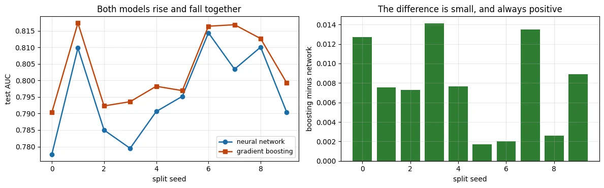
This is the heart of the note, so read the two panels together with the numbers above them.
Summarised separately, the two models are indistinguishable. The network averages 0.7956 with a standard deviation of 0.0132; boosting averages 0.8034 with 0.0111. The gap between the averages, 0.0078, is smaller than either spread. If you reported one sentence per model, you would have to say the comparison is inconclusive.
Paired, the difference is +0.0078 with a standard deviation of 0.0047, and boosting wins all ten splits. The left panel shows why: the two lines move up and down together, because a split that is hard for one model is hard for the other. Subtracting removes that shared movement, exactly as in the made-up example in Section 2.
So the honest statement is: gradient boosting is better here, by a small and consistent margin of about 0.008 AUC. Not "much better". Not "indistinguishable".
And there is a general lesson underneath it, which Module 3 could not have shown you with single runs: a difference smaller than the noise floor can still be real, as long as you measure it in a way that cancels the noise.
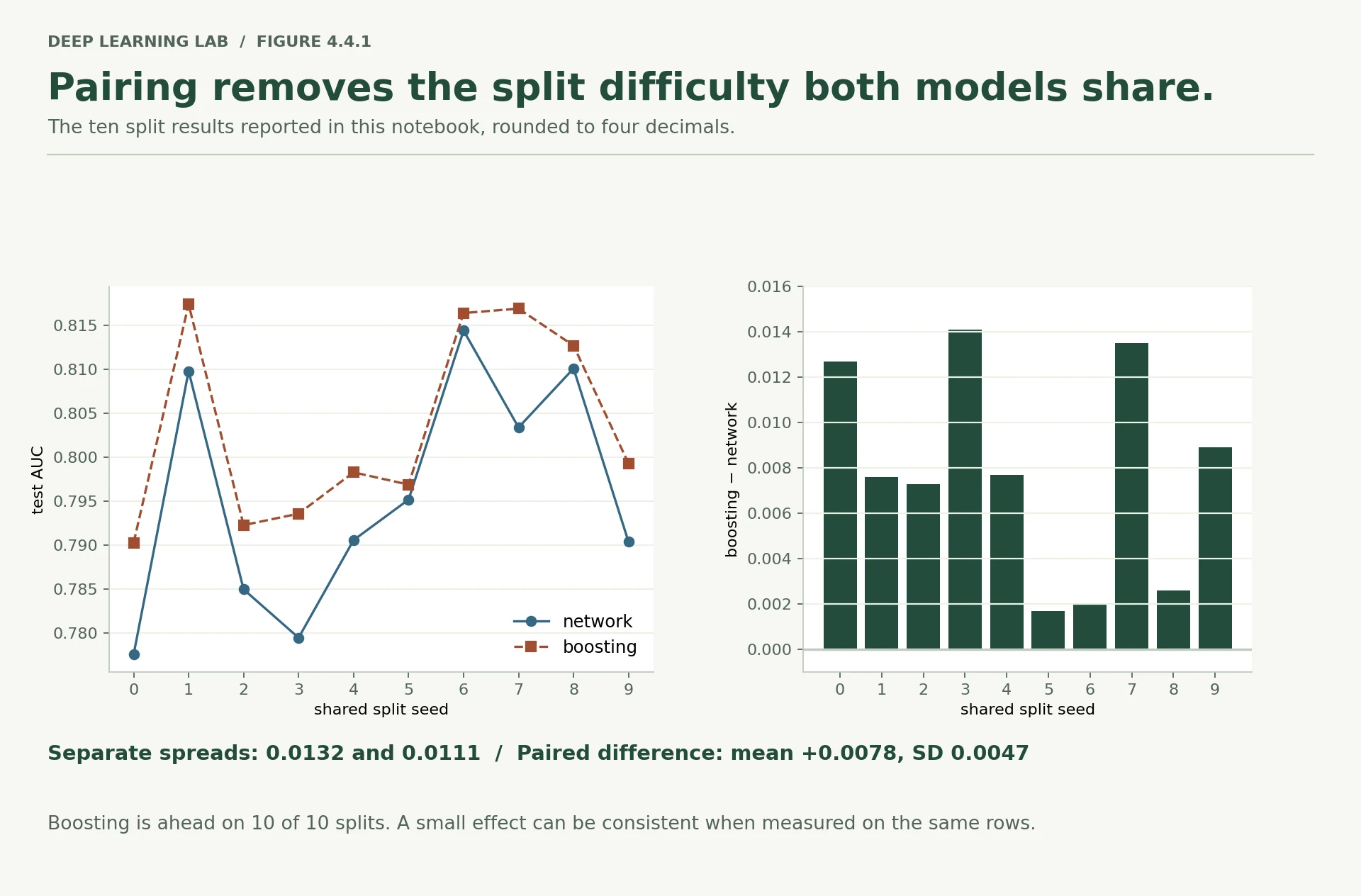
The ten real splits from the table above, drawn to the same scale in both panels. Every arrow points the same way, from wherever that split happened to sit.
Deep diveHow sure, in numbers, and a catch about repeated splits
The usual tests agree with the reading above:
| paired t-test | corrected for overlapping splits | sign test | |
|---|---|---|---|
| boosting minus network | t = 5.3, p = 0.0005 | t = 3.5, p = 0.006; 95% interval +0.003 to +0.013 | 10 of 10, p = 0.002 |
| tuned minus default | t = 1.5, p = 0.17 | t = 1.0, p = 0.35; 95% interval −0.002 to +0.004 | 5 of 10, p = 1.0 |
The catch: ten random splits of one file are not ten independent experiments. Any two share most of their training rows, so their results are correlated, and a plain t-test is too confident. Nadeau and Bengio (2003) proposed a simple fix: multiply the variance by \(1/k + n_\text{test}/n_\text{train}\) instead of \(1/k\) (here \(0.1 + 0.125\)). After it, boosting's advantage is still clearly real and the tuning gain still is not.
The fix also shows where more splits stop helping: the \(n_\text{test}/n_\text{train}\) term does not shrink with \(k\), so going from 10 splits to 30 narrows this interval by only about 16%, not the 42% that the square-root rule suggests.
-
In your own words: why is the spread of the difference smaller than the spread of either model?
Because most of each model's variation is not about the model; it is about the split. A test set full of easy customers lifts both scores, a hard one lowers both. That shared movement is identical for the two models on the same rows, so it vanishes when you subtract, and only each model's own wobble is left. In symbols, the variance of the difference is the sum of the two variances minus twice their covariance, and here the covariance is large.
-
Suppose boosting had won 6 splits out of 10 with the same average difference. What would you conclude?
That the average is not the whole story. With 6 wins in 10, the difference changes sign on four splits, so it is noisy compared with its mean, and a sign test on 6 of 10 gives p = 0.75: no evidence of a consistent advantage. Check whether one or two large splits are carrying the average. Under the rules of Section 1 the verdict is "within the noise", and the decision passes to the cost and robustness columns.
-
Would twenty more splits make the difference bigger? What would they improve?
No. The average difference estimates a fixed quantity (about 0.008 here), so more splits would not move it in any particular direction; they would pin it down more precisely, and give a better estimate of its spread. By the square-root rule, 30 splits instead of 10 would narrow the interval by about 42%. Because random splits of one file overlap, the real gain is smaller: about 16% by the correction in the note above. Twenty more splits would buy a little precision and no change of verdict.
Summarise a paired comparison
The lists hold test AUC for ten splits, both models on identical rows. Return the mean and standard deviation (with ddof=1) of the
split-by-split difference b − a, and the number of splits where b wins.
Each model's AUC varies by ~0.013 across splits, the gap between averages is 0.008, and boosting wins all ten paired splits. The verdict?
A difference smaller than the noise floor can still be real when you measure it in a way that cancels the noise.
Boosting wins 6 of 10 splits with the same average difference. What would you conclude, and why?
- Much weaker evidence: a 6–4 split is close to a coin toss, so the average may be driven by one or two large splits.
- You'd report 'no reliable difference' (or collect more splits/data), because consistency across paired splits is what made the 10–0 result convincing.
Does the tuning survive the noise?
The tuned settings won the search on validation. The rules said carry them to all ten splits, which we did. Now compare them with the untuned defaults, paired, exactly as before.
tuning_gain = bakeoff["boosting tuned"] - bakeoff["boosting"]print("tuned minus default, across ten splits:")print(f" average : {tuning_gain.mean():+.4f}")print(f" standard deviation : {tuning_gain.std(ddof=1):.4f}")print(f" tuned ahead on : {int((tuning_gain > 0).sum())} of 10 splits")print()print("on split 42, the one the search was scored on:")print(f" validation AUC : tuned {grid.val_auc.max():.4f} against default {gbdt_default['val_auc']:.4f}")print(f" test AUC : tuned {grid.iloc[0].test_auc:.4f} against default {gbdt_default['test']['auc']:.4f}")tuned minus default, across ten splits: average : +0.0012 standard deviation : 0.0024 tuned ahead on : 5 of 10 splits on split 42, the one the search was scored on: validation AUC : tuned 0.7994 against default 0.7944 test AUC : tuned 0.8109 against default 0.8160
The tuning moved the paired result by +0.0012, with a standard deviation of 0.0024, winning five splits out of ten. Five out of ten is a coin toss. The twelve-setting budget produced nothing.
The two lines underneath show how the illusion forms. On the split the search was scored on, the tuned settings beat the defaults on validation, 0.7994 against 0.7944 — exactly the kind of gain that gets written up. On the test rows of that same split they were worse, 0.8109 against 0.8160.
Picking the best of twelve noisy numbers partly picks luck, and luck does not transfer to new rows.
This is the same lesson Lesson 3.2 reached from the other direction, where eight different regularisation settings turned out to be indistinguishable once early stopping was in place. Searching a space of settings costs real time. Before spending it, check whether the space you are searching is wider than your noise. Here it was not: the whole search spanned 0.0068 and the split noise is 0.0130.
-
The tuned settings won on validation and lost on test, on the same split. What is the one-sentence explanation?
The search picked the setting with the highest validation score on split 42, part of that score was luck specific to those 4,521 rows, and the test rows of the same split do not share that luck, so the advantage vanished (here it even reversed).
-
What would make a twelve-setting search worth running on this dataset?
Candidates that really differ by more than the paired noise, and a way of scoring them that averages out luck. Concretely: settings that change the model substantially (much larger or smaller trees, very different numbers of trees, class weights, a different treatment of the categorical columns) rather than twelve close neighbours of the defaults; each candidate scored paired across several splits (as in Section 5) instead of on one validation set; or much more data, where validation noise is smaller. It also helps to decide beforehand how large a gain would be worth shipping, and ask whether the search could plausibly deliver it.
The best of twelve settings beat the default on validation, then lost on the test rows of the same split. Most likely?
Paired across ten splits, tuning gained +0.0012 ± 0.0024 and won 5 of 10. The budget produced nothing.
The cost column
Accuracy is one column of the decision. Here are the others, measured rather than assumed.
One caution about timing first, and it is the kind of thing that quietly makes comparisons unfair. Our network's timer covers 30 epochs including scoring the validation rows after each one, which is diagnostic work rather than training work. Gradient boosting's timer covers only its fit. To compare like with like, time the bare training loop as well.
split = split_42pre = build_preprocessor(X).fit(X.iloc[split["train"]])train_inputs = torch.tensor(pre.transform(X.iloc[split["train"]]).astype(np.float32))train_targets = torch.tensor(y[split["train"]]).unsqueeze(1)def bare_training_seconds(epochs=30): """Time the network's training loop alone, with no validation scoring between epochs. Uses the preprocessed rows of split 42 and the frozen Module 3 settings. Args: epochs: Passes over the training rows. Returns: Seconds spent in the training loop. """ torch.manual_seed(42) model = nn.Sequential(nn.Linear(train_inputs.shape[1], 64), nn.ReLU(), nn.Linear(64, 32), nn.ReLU(), nn.Linear(32, 1)) optimizer = torch.optim.AdamW(model.parameters(), lr=1e-3, weight_decay=0.0) loss_function = nn.BCEWithLogitsLoss() generator = torch.Generator().manual_seed(42) loader = torch.utils.data.DataLoader( torch.utils.data.TensorDataset(train_inputs, train_targets), batch_size=256, shuffle=True, generator=generator) started = time.perf_counter() for _ in range(epochs): for batch_x, batch_y in loader: optimizer.zero_grad() loss_function(model(batch_x), batch_y).backward() optimizer.step() return time.perf_counter() - startednetwork_training_seconds = bare_training_seconds()print(f"network, 30 epochs, training only : {network_training_seconds:.2f} s")print(f"network, as the run function reports it : {nn_reference['seconds']:.2f} s (scoring included)")print(f"gradient boosting, fit : {gbdt_default['seconds']:.2f} s")print(f"ratio, training only : {network_training_seconds / gbdt_default['seconds']:.1f}x")network, 30 epochs, training only : 6.80 s network, as the run function reports it : 7.19 s (scoring included) gradient boosting, fit : 0.49 s ratio, training only : 13.8x
Next, how long each one takes to make predictions, and how big each one is to ship.
Latency means the time to produce predictions, measured here for 1,000 raw customer rows, with the preprocessing included, because in production you have to do that too. We take the median of five attempts, because single timings are noisy.
def latency_ms_per_1000_rows(predict, raw_rows, repeats=5): """Median time to score 1,000 raw rows, preprocessing included. Args: predict: A function from raw rows (a DataFrame) to probabilities. raw_rows: At least 1,000 raw rows; the first 1,000 are used. repeats: How many timed attempts to take the median of. Returns: Milliseconds per 1,000 rows. """ sample = raw_rows.iloc[:1000] times = [] for _ in range(repeats): started = time.perf_counter() predict(sample) times.append(time.perf_counter() - started) return 1000 * float(np.median(times))network_model = nn_reference["artifacts"]["model"]network_preprocessor = nn_reference["artifacts"]["preprocessor"]def network_predict(raw_rows): """Score raw rows with the reference network: preprocess, forward pass, sigmoid. Args: raw_rows: A DataFrame of raw input columns. Returns: A NumPy array of probabilities, one row per input row. """ with torch.no_grad(): return torch.sigmoid(network_model( torch.tensor(network_preprocessor.transform(raw_rows).astype(np.float32)))).numpy()def boosting_predict(raw_rows): """Score raw rows with the default gradient-boosting model. Args: raw_rows: A DataFrame of raw input columns. Returns: A NumPy array with the probability of "yes" for each row. """ return gbdt_default["artifacts"]["model"].predict_proba(as_categorical(raw_rows))[:, 1]test_rows_raw = X.iloc[split["test"]]network_latency = latency_ms_per_1000_rows(network_predict, test_rows_raw)boosting_latency = latency_ms_per_1000_rows(boosting_predict, test_rows_raw)weights_buffer, preprocessor_buffer = io.BytesIO(), io.BytesIO()torch.save(network_model.state_dict(), weights_buffer)joblib.dump(network_preprocessor, preprocessor_buffer)network_bytes = weights_buffer.getbuffer().nbytes + preprocessor_buffer.getbuffer().nbytesprint(f"network : {network_latency:5.1f} ms per 1,000 rows | {network_bytes / 1024:5.0f} KB to ship")print(f"boosting : {boosting_latency:5.1f} ms per 1,000 rows | " f"{gbdt_default['artifact_bytes'] / 1024:5.0f} KB to ship")- 1
The median ignores one slow attempt, such as a first call paying for memory allocation.
- 2
Preprocessing is inside the timed call, because production has to do it too.
- 3
Safe even though the 1,000 rows may lack some categories: the model maps values by name to what it saw in training.
network  :   6.1 ms per 1,000 rows |    28 KB to ship
boosting :  13.4 ms per 1,000 rows |   344 KB to ship
cost_table = pd.DataFrame([ {"": "test AUC over 10 splits", "neural network": f"{bakeoff.network.mean():.4f} ± {bakeoff.network.std(ddof=1):.4f}", "gradient boosting": f"{bakeoff.boosting.mean():.4f} ± {bakeoff.boosting.std(ddof=1):.4f}"}, {"": "training time (seconds)", "neural network": f"{network_training_seconds:.2f}", "gradient boosting": f"{gbdt_default['seconds']:.2f}"}, {"": "prediction, ms per 1,000 rows", "neural network": f"{network_latency:.1f}", "gradient boosting": f"{boosting_latency:.1f}"}, {"": "size to ship (KB)", "neural network": f"{network_bytes / 1024:.0f}", "gradient boosting": f"{gbdt_default['artifact_bytes'] / 1024:.0f}"}, {"": "preparation needed", "neural network": "scale + one-hot, 15 columns -> 50", "gradient boosting": "mark categories, 15 columns"}, {"": "files to ship", "neural network": "weights + fitted preprocessor", "gradient boosting": "one model file"}, {"": "settings that matter", "neural network": "learning rate, epochs, width, batch size, regularisation", "gradient boosting": "learning rate, leaves, number of trees"}, {"": "does a GPU help?", "neural network": "yes, at larger scale", "gradient boosting": "no"},])print(cost_table.to_string(index=False)) neural network gradient boosting
test AUC over 10 splits 0.7956 ± 0.0132 0.8034 ± 0.0111
training time (seconds) 6.80 0.49
prediction, ms per 1,000 rows 6.1 13.4
size to ship (KB) 28 344
preparation needed scale + one-hot, 15 columns -> 50 mark categories, 15 columns
files to ship weights + fitted preprocessor one model file
settings that matter learning rate, epochs, width, batch size, regularisation learning rate, leaves, number of trees
does a GPU help? yes, at larger scale no
Read that as a set of trades rather than a scoreboard.
Training. Boosting fits in 0.49 seconds against 6.80 for the network's 30 epochs — about 14 times faster on the same machine — with no epoch count to choose and no learning rate to get wrong.
Prediction. The network is the faster one here, 6.1 ms per 1,000 rows against 13.4, because scoring it is a few small matrix multiplications while boosting has to walk dozens of trees. Its files are also far smaller, 28 KB against 344 KB.
Everything else. The network needs a fitted preprocessor that has to be saved, versioned and kept in step with the weights — which is exactly what Lesson 4.2's bundle existed to manage. Boosting ships one file and takes the raw columns.
At this volume of requests none of the prediction numbers is a constraint, which is why the accuracy and training columns carry the decision. At a hundred thousand requests a second, or on a device with a hard size limit, the same table would point the other way.
-
The run function's timer included scoring. Name another way a timing comparison can quietly become unfair.
Any of these:
- Threads. scikit-learn's histogram boosting uses every CPU core through OpenMP by default, while PyTorch uses its own thread setting (Lesson 4.3's machine reported one thread). Record the thread counts, and equalise them if you can.
- Stopping rules. Boosting stopped when its held-out loss stopped improving (75 trees). The network always ran all 30 epochs, although its best epoch across the ten splits was between 8 and 22; with early stopping its time would fall by a third or more.
- Warm-up. The first call pays one-off costs (memory allocation, lazy initialisation). Time several repeats after a warm-up and take the median, as the latency cell does.
- Different hardware for the two sides, or data preparation inside one timer and outside the other.
-
At what dataset size would you expect the training-time ratio to start favouring the network?
Perhaps never, on a CPU and for data like this: both training costs grow roughly in proportion to the number of rows, so the ratio stays similar as the data grows. What changes it lies elsewhere. A network on a GPU against boosting on a CPU (though XGBoost, LightGBM and CatBoost can also train on GPUs; the table's "no" is true of scikit-learn's implementation). Very large datasets, where a network may need only one or two passes. And, above all, inputs such as text, images or audio, where boosting first needs features built by hand. The crossover point is something to measure on your data, not to assume.
Which timing comparison is fair?
The run function's timer included scoring, which is diagnostic work. Bare training: 6.80 s vs 0.49 s (~14×).
Which cost favoured the network?
At this request volume neither latency matters; at 100k requests per second, or on a small device, the same table could point the other way.
List three non-accuracy columns that belong in a model decision, with this lesson's example for each.
- Training time (boosting ~14× faster, no epochs or learning rate to choose); prediction latency and model size (network faster and smaller).
- Preparation and moving parts (the network needs a fitted preprocessor kept in step with its weights); behaviour under shift (Section 8).
The robustness column
Everything so far used the stratified split, which answers "how well on a random customer from 2008 to 2010?". Lesson 4.1 showed that the deployment question is different, and that the chronological split answers it: train on the earliest 80% of the file, test on the last 10%, where 47% of customers say yes.
Run both models there.
chronological = { "network": run_neural_network({"name": "bake_nn_chrono", "split": "chronological"}, quiet=True), "boosting": run_gradient_boosting({"name": "bake_gbdt_chrono", "split": "chronological"}, quiet=True), "boosting tuned": run_gradient_boosting({"name": "bake_tuned_chrono", "split": "chronological", **TUNED}, quiet=True),}comparison = pd.DataFrame([ {"model": name, "stratified test AUC": bakeoff[name].mean() if name in bakeoff else np.nan, "chronological test AUC": result["test"]["auc"], "average prediction": result["test"]["average_prediction"], "share who actually said yes": result["test"]["share_who_said_yes"]} for name, result in chronological.items()])print(comparison.round(4).to_string(index=False))print()print(f"network's best epoch under the chronological split: " f"{chronological['network']['best_epoch']} (it was {nn_reference['best_epoch']} on the stratified one)") model stratified test AUC chronological test AUC average prediction share who actually said yes
network 0.7956 0.6141 0.1284 0.4709
boosting 0.8034 0.5841 0.1863 0.4709
boosting tuned 0.8046 0.5714 0.1771 0.4709
network's best epoch under the chronological split: 2 (it was 18 on the stratified one)
Both models fall a long way, and the ranking reverses. The network, which lost on every stratified split, is now the better of the two.
Before making anything of that, notice the problem: this is one test set, not ten. Time only runs in one direction, so there is no second chronological split to compare against.
The tool for that situation is the bootstrap. The idea is simple: treat your test set as a stand-in for the population, and draw a new test set from it with replacement — meaning the same row can be drawn twice, and some rows not at all. Score both models on that resample. Do it a thousand times, and the spread of the differences tells you how much your single result depends on which particular rows you happened to have.
network_probabilities = chronological["network"]["artifacts"]["test_probabilities"]boosting_probabilities = chronological["boosting"]["artifacts"]["test_probabilities"]chronological_labels = y[chronological["network"]["artifacts"]["split"]["test"]]point_estimate = (roc_auc_score(chronological_labels, network_probabilities) - roc_auc_score(chronological_labels, boosting_probabilities))generator = np.random.default_rng(0)n_rows = len(chronological_labels)differences = []for _ in range(1000): picked = generator.integers(0, n_rows, n_rows) # draw n rows, with replacement if chronological_labels[picked].sum() in (0, len(picked)): continue # skip a resample with only one class differences.append(roc_auc_score(chronological_labels[picked], network_probabilities[picked]) - roc_auc_score(chronological_labels[picked], boosting_probabilities[picked]))differences = np.array(differences)low, high = np.percentile(differences, [2.5, 97.5])print(f"chronological split, network minus boosting")print(f" measured on the real test rows : {point_estimate:+.4f}")print(f" 95% of resamples fall between : {low:+.4f} and {high:+.4f}")print(f" resamples where the network is ahead: {(differences > 0).mean():.1%}")- 1
Some rows are drawn twice and about 37% not at all; each resample is a plausible other test set.
- 2
AUC needs both classes; with 4,521 rows this never actually triggers.
- 3
Both models are scored on the same resample, so the bootstrap is paired too.
- 4
The percentile interval: the middle 95% of the resampled differences.
chronological split, network minus boosting
  measured on the real test rows : +0.0300
  95% of resamples fall between  : +0.0172 and +0.0437
  resamples where the network is ahead: 100.0%
The network is ahead by 0.0300, and the interval from +0.0172 to +0.0437 does not include zero, with the network ahead in 100% of the resamples. So the reversal is not an accident of which rows landed in that one test set.
Notice how much larger this gap is than the 0.0078 that separated the models on the stratified splits. The shift changed the ranking by roughly four times the margin the original comparison was arguing about.
The network's best epoch also moved, from 18 down to 2. Its validation rows now come from a later, different period, so the run reaches its best general performance almost immediately and then spends 28 more epochs fitting itself more tightly to a training period that no longer describes the world.
Why would the more flexible model suffer more? Because flexibility is fitted to the training distribution. Gradient boosting carves the old population into many fine regions, and when the population moves, a lot of those regions no longer describe anybody. The smaller, smoother model has less to be wrong about. That is a pattern worth carrying forward, not a fact about these two libraries.
And be careful what this does not say. It does not say the network is fit to deploy. Both models lose most of their skill, and both are badly miscalibrated on the later period, predicting far below the true rate of 47%. The honest conclusion is that the shift is the dominant problem, and it is bigger than the choice of model.
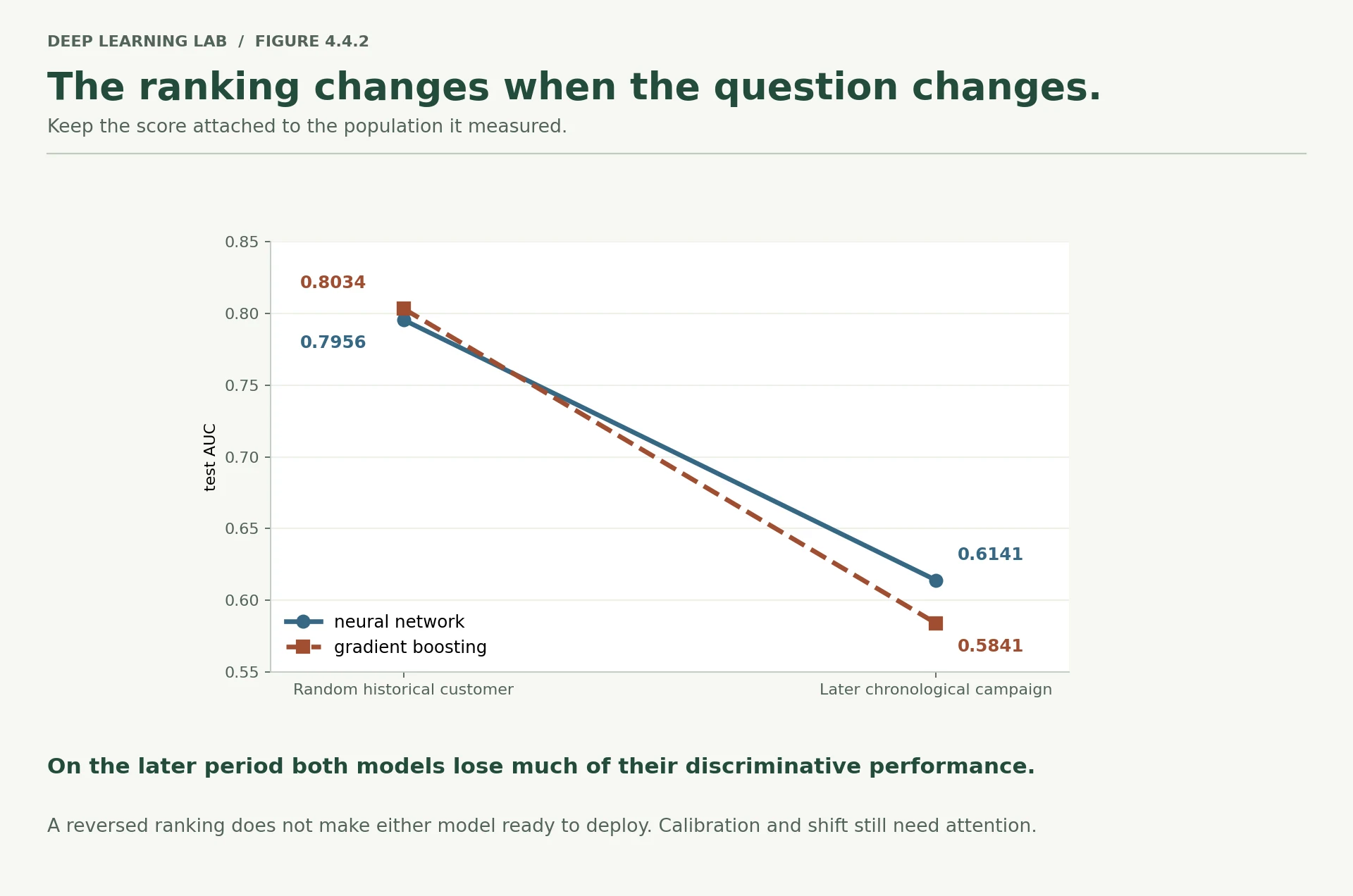
Stratified values are the ten-split averages; chronological values are the single later-period test set. The lines cross, and both end close to guessing.
-
Why bootstrap the test rows here instead of running ten chronological splits?
Because there is only one chronological split to run. "Train on the past, test on the future" fixes the cut-off, so the test rows are the same every time; the only randomness left in the evaluation is which rows happened to land in that test period, and the bootstrap measures exactly that. (A related tool, rolling-origin evaluation, trains and tests at several cut-off dates. It answers a different question: whether the ranking holds across periods.)
-
The interval covers the wobble from which rows you tested on. Name a source of uncertainty it does not cover.
Anything that would change the models rather than the test rows: the training randomness (both fitted models are held fixed in every resample), which rows ended up in training and validation, and the choice of cut-off date. It also does not cover the next period being different again. And one limitation affects the interval itself: the bootstrap treats rows as independent, but calls made on the same day or in the same campaign are alike (Lesson 4.1 found day-level success rates varying enormously). Resampling whole days rather than rows would give a wider, more honest interval.
-
Both models are badly calibrated on the later period. What would you do about that before shipping either?
Recalibrate on recent labelled data: fit a small calibration step (Platt scaling or isotonic regression) on the most recent period, or retrain with recent rows included. The share who said yes moved from about 12% across the file to 47% in the test period, so even shifting the model's intercept by the change in log-odds would remove much of the error. Calibration leaves the ranking, and so the AUC, unchanged; it fixes the probabilities, which matter as soon as anyone reads them as chances or puts a threshold on them. If the threshold comes from calling capacity (Lesson 4.1 Section 10), the ranking is what counts. Then keep checking calibration as each new month of outcomes arrives.
In Section 8's bootstrap, what is resampled?
Time runs one way, so there is only one chronological test set; the bootstrap shows how much the result depends on which rows were in it.
Under the chronological split, the ranking reversed (network ahead by 0.030). What is the honest conclusion?
The shift changed the ranking by about four times the stratified margin. Flexibility fitted to the old population suffers more when it moves.
The bootstrap interval covers which rows you tested on. Name a source of uncertainty it does not cover.
- It does not cover training randomness (seed), the choice of training/validation period, or future periods that differ from this one.
- It also can't tell you how the shift will continue: one later period is one sample of 'the future'.
Where the two models disagree
Two models with nearly the same AUC are not necessarily making the same predictions. On the stratified split, compare them customer by customer.
Spearman correlation measures whether two sets of scores put things in the same order, ignoring the actual values. 1.0 means identical order; 0 means no relationship.
from scipy.stats import spearmanrnetwork_test = nn_reference["artifacts"]["test_probabilities"]boosting_test = gbdt_default["artifacts"]["test_probabilities"]labels_test = y[split["test"]]print(f"how similarly they rank customers (Spearman): {spearmanr(network_test, boosting_test)[0]:.4f}")print(f"neural network AUC : {roc_auc_score(labels_test, network_test):.4f}")print(f"gradient boosting AUC : {roc_auc_score(labels_test, boosting_test):.4f}")print(f"the two averaged : {roc_auc_score(labels_test, (network_test + boosting_test) / 2):.4f}")how similarly they rank customers (Spearman): 0.8658 neural network AUC : 0.8016 gradient boosting AUC : 0.8160 the two averaged : 0.8163
slices = { "contacted in an earlier campaign": (test_rows_raw.pdays > -1).to_numpy(), "never contacted before": (test_rows_raw.pdays == -1).to_numpy(), "contact type known": (test_rows_raw.contact != "unknown").to_numpy(), "contact type unknown": (test_rows_raw.contact == "unknown").to_numpy(),}slice_rows = []for name, mask in slices.items(): slice_rows.append({"slice": name, "rows": int(mask.sum()), "share who said yes": labels_test[mask].mean(), "network AUC": roc_auc_score(labels_test[mask], network_test[mask]), "boosting AUC": roc_auc_score(labels_test[mask], boosting_test[mask])})slice_table = pd.DataFrame(slice_rows)slice_table["boosting minus network"] = slice_table["boosting AUC"] - slice_table["network AUC"]print(slice_table.round(4).to_string(index=False)) slice rows share who said yes network AUC boosting AUC boosting minus network
contacted in an earlier campaign 843 0.2444 0.8547 0.8640 0.0093
never contacted before 3679 0.0878 0.7478 0.7675 0.0198
contact type known 3187 0.1490 0.7984 0.8156 0.0172
contact type unknown 1335 0.0404 0.6246 0.6210 -0.0036
The two models rank customers similarly but not identically: a Spearman correlation of 0.8658. Averaging their predictions gives 0.8163 against boosting's 0.8160, so combining them bought nothing worth shipping a second model for.
The slices are more useful. Boosting is ahead on three of the four, and its biggest advantage is on customers never contacted before (+0.0198), which is also the largest and hardest slice — its ability to carve up the raw categorical columns evidently helps there. On customers whose contact type is unknown, the two are level (−0.0036), and that slice is where both models are weakest in absolute terms: 0.6246 for the network and 0.6210 for boosting, against 0.75 to 0.86 everywhere else.
That slice was flagged in Lesson 4.1 as a suspicious 28.8% of rows with a low success rate, and Lesson 4.1 Section 8 found it shrinking sharply over time. Neither model solves it, and no amount of model choice will. That is a data question, and it is the kind of thing Module 9's error analysis is built to chase.
Deep diveHow much of a slice table is noise?
Every number in the slice table comes from one split, and some slices have few positives: 206 in contacted in an earlier campaign, 323 in never contacted before, 475 in contact type known, and only 54 in contact type unknown. By the Hanley–McNeil approximation, a single AUC measured on those rows has a standard error of about 0.017, 0.016, 0.013 and 0.041. That is as large as most of the differences in the last column.
The difference between two models on the same rows is less noisy than either AUC, because their errors are correlated, but only resampling says by how much. Run Section 8's paired bootstrap inside each slice, or repeat the slice table on the ten splits of Section 5. The reading that survives either check is the big one: both models are far weaker on contact type unknown (about 0.62, against 0.75 to 0.86 elsewhere). Which model leads inside a slice is much less certain.
The two models rank customers with Spearman 0.87, and averaging them gives 0.8163 against 0.8160. What follows?
Slices are more useful: both are weakest on contact == 'unknown', a data question no model choice fixes.
The decision memo
The blueprint asks for a decision rule, not a winner. Here is the memo, written from the measurements above, and then a short record for each side in the Lesson 4.2 format.
memo = f"""# Decision memo: model choice for Bank Marketing subscription prediction## RecommendationShip **gradient boosting** (HistGradientBoostingClassifier, default settings) for this problemat this size, and treat the distribution shift as more urgent than the choice of model.## Evidence- Accuracy, 10 paired stratified splits: boosting {bakeoff.boosting.mean():.4f} against network {bakeoff.network.mean():.4f}. Paired difference {difference.mean():+.4f} (standard deviation {difference.std(ddof=1):.4f}), boosting ahead on {int((difference > 0).sum())} of 10 splits. Small, consistent, real.- Tuning: a twelve-setting search changed the paired result by {tuning_gain.mean():+.4f} (standard deviation {tuning_gain.std(ddof=1):.4f}), ahead on {int((tuning_gain > 0).sum())} of 10. Not worth the budget.- Cost: trains {network_training_seconds / gbdt_default['seconds']:.0f}x faster, with no scaling or one-hot pipeline to fit, maintain and ship. Predictions are slower per 1,000 rows ({boosting_latency:.1f} ms against {network_latency:.1f} ms) and the file is larger ({gbdt_default['artifact_bytes'] / 1024:.0f} KB against {network_bytes / 1024:.0f} KB); at this request volume neither is a constraint.- Robustness: under a chronological split both models collapse (boosting {chronological['boosting']['test']['auc']:.4f}, network {chronological['network']['test']['auc']:.4f}) and the ranking reverses, with a bootstrap interval that excludes zero. Neither is calibrated for the later period.## What would change this recommendation- Much more data, or raw text, image, audio or sequence inputs: revisit. That is where neural networks win, and it is what Days 5 to 9 are about.- A need to fine-tune a pretrained model, or to share an encoder with another task: gradient boosting cannot do either.- Prediction budgets in the low milliseconds per 1,000 rows, or a hard file-size limit.## Conditions on deployment- Retrain on a schedule. The success rate moved about tenfold across this file.- Watch the input distribution (Note 4.1's adversarial check) and recalibrate on recent data.- Choose the decision threshold from calling capacity, not from 0.5 (Note 4.1 Section 10).## Limitations- One dataset, one size, tabular only. This is not a general claim about model families.- The network's settings came from two days of tuning in Notes 2.3 to 3.4; boosting got twelve settings. The imbalance favours the network, and it still lost.- The chronological result is a single split; its bootstrap interval is in results/."""os.makedirs("results", exist_ok=True)with open("results/decision_memo.md", "w") as f: f.write(memo)print(memo)# Decision memo: model choice for Bank Marketing subscription prediction ## Recommendation Ship **gradient boosting** (HistGradientBoostingClassifier, default settings) for this problem at this size, and treat the distribution shift as more urgent than the choice of model. ## Evidence - Accuracy, 10 paired stratified splits: boosting 0.8034 against network 0.7956. Paired difference +0.0078 (standard deviation 0.0047), boosting ahead on 10 of 10 splits. Small, consistent, real. - Tuning: a twelve-setting search changed the paired result by +0.0012 (standard deviation 0.0024), ahead on 5 of 10. Not worth the budget. - Cost: trains 14x faster, with no scaling or one-hot pipeline to fit, maintain and ship. Predictions are slower per 1,000 rows (13.4 ms against 6.1 ms) and the file is larger (344 KB against 28 KB); at this request volume neither is a constraint. - Robustness: under a chronological split both models collapse (boosting 0.5841, network 0.6141) and the ranking reverses, with a bootstrap interval that excludes zero. Neither is calibrated for the later period. ## What would change this recommendation - Much more data, or raw text, image, audio or sequence inputs: revisit. That is where neural networks win, and it is what Days 5 to 9 are about. - A need to fine-tune a pretrained model, or to share an encoder with another task: gradient boosting cannot do either. - Prediction budgets in the low milliseconds per 1,000 rows, or a hard file-size limit. ## Conditions on deployment - Retrain on a schedule. The success rate moved about tenfold across this file. - Watch the input distribution (Note 4.1's adversarial check) and recalibrate on recent data. - Choose the decision threshold from calling capacity, not from 0.5 (Note 4.1 Section 10). ## Limitations - One dataset, one size, tabular only. This is not a general claim about model families. - The network's settings came from two days of tuning in Notes 2.3 to 3.4; boosting got twelve settings. The imbalance favours the network, and it still lost. - The chronological result is a single split; its bootstrap interval is in results/.
And the records, in the five-question format from Lesson 4.2. The function is repeated here so this notebook stands alone.
def experiment_record(result, why, learned, next_change, results_dir="results"): """Write ``<results_dir>/<name>.md``: the five questions every experiment should answer. Args: result: A result dict from ``run_neural_network`` or ``run_gradient_boosting``. why: Why the experiment was run; only a person can supply this. learned: What it taught; only a person can supply this. next_change: What to change next. results_dir: Folder for the record. Returns: The path of the Markdown file written. Raises: ValueError: If ``why`` or ``learned`` is empty. """ if not why or not learned: raise ValueError("a record needs both a reason and a lesson") test = result["test"] text = f"""### Experiment: {result['name']}model: {result['model']} · settings: `{result['settings']}`**1. What did I try?** {result['model']} on Bank Marketing, stratified split, seed{result['settings']['split_seed']}.**2. Why?** {why}**3. What happened?** validation AUC {result['val_auc']:.4f}; test AUC {test['auc']:.4f},test PR-AUC {test['pr_auc']:.4f} (share who said yes {test['share_who_said_yes']:.3f});{result['seconds']:.2f} seconds to fit.**4. What did I learn?** {learned}**5. What would I change next?** {next_change}Full numbers: `{results_dir}/{result['name']}.json`""" path = os.path.join(results_dir, f"{result['name']}.md") with open(path, "w") as f: f.write(text) return pathexperiment_record( nn_reference, why=("The Day 3 network, frozen, should be competitive with gradient boosting on this " "tabular dataset. The blueprint warns that it may not win."), learned=(f"It lost on all ten paired splits, by {abs(difference.mean()):.4f} AUC on average. " f"That margin is smaller than the 0.013 split noise but consistent in direction. " f"It was the more robust of the two under the chronological split."), next_change=("Repeat the comparison on a dataset with raw text or sequence inputs, where the " "advantage of learned representations should show."))path = experiment_record( gbdt_default, why="Default gradient boosting should be a strong baseline on tabular data with no tuning.", learned=(f"Confirmed: defaults reached {gbdt_default['test']['auc']:.4f} test AUC in " f"{gbdt_default['seconds']:.2f} seconds with no preprocessing, and a twelve-setting " f"search added {tuning_gain.mean():+.4f} across splits, which is noise."), next_change="Try LightGBM and XGBoost on the same splits for a like-for-like check.")print(open(path).read())- 1
Refuses to write a record with the two answers only a person can supply (Lesson 4.2).
### Experiment: bakeoff_gbdt_42

model: gradient boosting · settings: `{'name': 'bakeoff_gbdt_42', 'split': 'stratified', 'split_seed': 42, 'seed': 42, 'learning_rate': 0.1, 'max_leaf_nodes': 31, 'l2_regularization': 0.0, 'max_iter': 100, 'early_stopping': 'auto'}`

**1. What did I try?** gradient boosting on Bank Marketing, stratified split, seed
42.

**2. Why?** Default gradient boosting should be a strong baseline on tabular data with no tuning.

**3. What happened?** validation AUC 0.7944; test AUC 0.8160,
test PR-AUC 0.4944 (share who said yes 0.117);
0.49 seconds to fit.

**4. What did I learn?** Confirmed: defaults reached 0.8160 test AUC in 0.49 seconds with no preprocessing, and a twelve-setting search added +0.0012 across splits, which is noise.

**5. What would I change next?** Try LightGBM and XGBoost on the same splits for a like-for-like check.

Full numbers: `results/bakeoff_gbdt_42.json`
records = sorted(f for f in os.listdir("results") if f.endswith(".md"))results = sorted(f for f in os.listdir("results") if f.endswith(".json"))print(f"{len(results)} result files and {len(records)} written records in results/")print("records:", records)50 result files and 5 written records in results/ records: ['bakeoff_gbdt_42.md', 'bakeoff_nn_42.md', 'data_card_bank_marketing.md', 'decision_memo.md', 'weights_only.md']
What does the blueprint ask the decision memo to deliver?
Here: ship gradient boosting for this problem at this size, and treat the distribution shift as more urgent than model choice.
Your turn
Three extensions, in increasing order of effort. Each one follows the same rules: declare the budget first, use the same splits, report the paired difference against the noise, and write the record.
- A third model. Add logistic regression to the ten-split comparison. Lesson 3.1 reported 0.7717 for it on the Module 2 split. Does it survive a paired comparison against the other two, and what does its cost column look like?
- The imbalance question. Run the network with
pos_weightset to 7.5, roughly the ratio of no answers to yes answers, across the same ten splits. Lesson 4.1 Section 10 predicts the ranking will not change. Check it, and check the calibration too. - Combining them. Section 9 averaged the two models on one split. Does the average beat the better model across all ten, paired? If it does, is the gain worth shipping two models and maintaining both?
# Scratch space for your extensions.# for seed in range(10):# ...print("ready")ready
What to take away
Write the rules before the first result. The measure, the splits, the tuning budget, the decision rule, and what would change your mind. A comparison without them measures effort, not models.
Compare on identical rows and look at the paired difference. A gap smaller than the noise floor can still be real, and a gap larger than it can still be luck if the two models saw different rows.
Check tuning gains against the noise. Twelve settings spanning less than the split noise cannot produce a finding, however carefully you rank them.
Accuracy is one column. Training time, prediction time, file size, preparation needed, the number of things that can break in production, and behaviour under shift all belong in the decision.
Test the deployment condition, not just the convenient one. The ranking reversed under the chronological split, and both models lost most of their skill. That finding matters more than the 0.008 that separated them.
On tabular data of this size, gradient boosting is the baseline to beat. Deep learning's advantage is learning representations from raw inputs — text, images, audio, sequences — which is exactly where Modules 5 to 9 go.
Where Module 4 leaves you
Across the four notes you have built the engineering layer the rest of the course runs on:
4.1  data you can trust      audit, split rules and a contract, leakage measured three ways
4.2  experiments you can     seeds, settings, records, checkpoints that resume,
     reproduce               and the size of the noise
4.3  memory and precision    what a run costs before you start it, and the OOM playbook
4.4  the bake-off            a controlled comparison with error bars, cost, robustness,
                             and a written decision
That is the blueprint's Module 4 competency: conduct and communicate a defensible Deep Learning experiment.
Transition to Module 5
Module 4's conclusion also points straight at Module 5. Gradient boosting won on 15 tabular columns that people had already engineered into something useful. It has no answer at all when the input is a sentence, a photograph or a recording, because there is nothing to split on until somebody builds features by hand.
That gap is exactly what representation learning fills. Module 5 asks how a network turns raw input into a representation that makes a task easy, what an embedding is, how similarity works in that space, and how CLIP puts a picture and a sentence into the same space. From there, Module 6 opens the architecture that learns the best representations we currently have: the Transformer.
Why is ten random splits of one file weaker evidence than ten independent datasets?
Splits measure noise within one dataset; independent datasets would test whether the conclusion transfers.
Wrap-up
- Write the rules before the first result: the question, the splits, the measure, the tuning budget, the decision rule and what would change your mind.
- Compare on identical rows and read the paired difference. Each model alone spread by 0.013; their difference by 0.005, with boosting ahead on 10 of 10 splits.
- Random splits of one file overlap, so a plain paired test is too confident. Corrected, boosting's +0.008 still holds (95% interval +0.003 to +0.013).
- Judge tuning the same way: paired, across splits. The best of twelve settings on one validation set won by luck and added +0.001, winning 5 of 10.
- Accuracy is one column. Boosting trained 14 times faster and ships as one file; the network predicted twice as fast from a file twelve times smaller.
- Test the deployment condition. Chronologically the ranking reversed (network +0.030, interval +0.017 to +0.044) and both models fell towards guessing. Before explaining a reversal, check that both models saw the same information.
- On tabular data of this size, gradient boosting is the baseline to beat. Networks earn their place when they learn representations from raw text, images, audio and sequences.
Quick check
Two models are scored on the same ten splits. Why is the spread of their difference much smaller than either model's spread?
Here the two models' scores correlate at 0.94 across splits.
Each model's test AUC varies by 0.013 across splits; the gap between their averages is 0.008, and one wins on all ten paired splits. The verdict?
A gap smaller than the spread of single scores can still be real when the paired difference is consistent.
The best of twelve settings beat the default on validation, then lost on the test rows of the same split. Most likely?
Across ten splits the tuned setting added +0.0012 and won 5 of 10: a coin toss.
In Section 8's bootstrap, what is resampled?
So the interval covers which test rows you happened to have, not training randomness.
Why is ten random splits of one file weaker evidence than ten independent datasets?
Hence the corrected test, and why more splits stop narrowing the interval.
The two models rank customers with a Spearman correlation of 0.87, and averaging them gives 0.8163 against 0.8160. What follows?
Not worth maintaining a second model on this evidence; check it paired across splits before deciding.
Under the chronological split the network picked its epoch on the later-period validation rows, while boosting stopped using a slice of its training rows. Why does that matter?
Give both models the same information before crediting the reversal to smoothness.
Questions and discussion
Ask about this lesson, share what you found in a lab, or help someone else. Posts are public on the course's GitHub Discussions: anyone can read them, and you need a GitHub account to post.
Opening it loads giscus from giscus.app.