Module 6 · Transformers and Attention Mechanisms Lesson 6.4

The Transformer Block

Classroom material

33 min · 12 code cells · 1 labs

In this lesson

Time: ~33 min
Sections: 10
Code cells: 12
Labs: 1
Figures: 6

Start the lesson

Before you start

What is inside a Transformer block, and why does each part matter?

You will be able to: describe the four ingredients of a Transformer block and the job of each;
explain what the feed-forward network does and why it works on each token separately;
explain how residual connections help information and gradients flow, with measurements;
compute layer normalisation by hand;
explain the difference between post-norm and pre-norm blocks, and test how it matters in a specified training setup;
explain why stacking blocks increases what a model can represent.

In Lesson 6.3 we built multi-head causal self-attention, the part of a Transformer where tokens exchange information. But attention on its own is not a Transformer layer. Every Transformer stacks a repeated unit, the Transformer block, and attention is only one of its four ingredients. The other three (a feed-forward network, residual connections and layer normalisation) are less glamorous, but without them a deep Transformer would not train at all.

This lesson assembles the block, explains what each ingredient contributes, and then puts two of them to the test. We will see what happens to a 6-block model when its residual connections are removed, and we will reproduce one of the most important practical discoveries about Transformers: that where you put layer normalisation can strongly affect training stability, together with the learning rate and warmup.

Key question: What is inside a Transformer block, and why does each part matter?

Prerequisites

read Lesson 6.3. You should be comfortable with the training loop and with reading loss curves (Module 3).

Setup — imports, versions and device detection used by the notebook (1 cells)

Run this cell first. Most of this lesson runs instantly. The training experiments in Sections 6 and 7 take about two minutes in total on a CPU.

Environment and results. The saved outputs record one CPU reference run; random seeds reduce variation but do not guarantee identical numbers across computers. Read the comparisons as evidence from that run. Training times depend on your hardware.

If packages are missing, install them into your notebook environment, then restart the kernel and run from the beginning:

%pip install torch==2.14.1 numpy==2.5.4 pandas==3.0.6 matplotlib==3.11.2 scikit-learn==1.9.1 scipy==1.18.1

Setup 8 lines

import os, math, time, urllib.requestimport numpy as npimport torchimport torch.nn as nnimport torch.nn.functional as Fimport matplotlib.pyplot as plttorch.manual_seed(0)print("PyTorch", torch.__version__)

import os, math, time, urllib.request
import numpy as np
import torch
import torch.nn as nn
import torch.nn.functional as F
import matplotlib.pyplot as plt
torch.manual_seed(0)
print("PyTorch", torch.__version__)

Output

PyTorch 2.14.1+cu130

The Big Picture: How a Transformer Block Works

A Transformer block takes a sequence of token vectors and returns a sequence of the same shape, (batch, tokens, d_model), with each vector improved. It does that in two sub-layers, each wrapped in the same pattern:

Attention sub-layer: normalise the vectors, let tokens exchange information with multi-head self-attention, and add the result back to the input.
Feed-forward sub-layer: normalise again, process each token separately with a small two-layer network, and add the result back.

So the four ingredients are multi-head self-attention, a feed-forward network, residual connections (the "add back" steps) and layer normalisation (the "normalise" steps). In code, the modern version of the block is just two lines:

x = x + attention(layer_norm_1(x))
x = x + feed_forward(layer_norm_2(x))

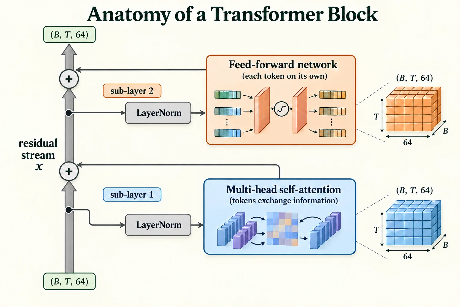
Anatomy of a Transformer Block. The pre-norm block adds attention and feed-forward updates to the residual stream, with LayerNorm on each branch.

Figure 6.4.1. The pre-norm block adds attention and feed-forward updates to the residual stream, with LayerNorm on each branch. Every stage preserves (B, T, 64). The feed-forward network is shared across positions.

Here is the block in PyTorch, built from the attention module of Lesson 6.3. It has two switches that we will use for experiments later: pre_norm chooses where layer normalisation goes, and residual lets us remove the "add back" steps.

Python 81 lines

class CausalSelfAttention(nn.Module):    """Projected multi-head self-attention with a causal mask and output projection."""    def __init__(self, d_model, n_heads):        """Create the components of this model; the forward computation is traced in the lesson.        Arguments:            d_model: Feature width of each token vector.            n_heads: Number of attention heads; divides model width.        """        super().__init__()        self.n_heads, self.d_head = n_heads, d_model // n_heads        self.qkv = nn.Linear(d_model, 3 * d_model)        self.proj = nn.Linear(d_model, d_model)    def forward(self, x):        """Projected multi-head self-attention with a causal mask and output projection.        Arguments:            x: Floating-point tensor; image models use (B, C, H, W), token-vector models use (B, T, D).        """        B, T, D = x.shape        q, k, v = self.qkv(x).split(D, dim=2)        q, k, v = [t.view(B, T, self.n_heads, self.d_head).transpose(1, 2) for t in (q, k, v)]        out = F.scaled_dot_product_attention(q, k, v, is_causal=True)      # (B, H, T, d_head)        return self.proj(out.transpose(1, 2).reshape(B, T, D))class FeedForward(nn.Module):    """Shared per-token nonlinear network expanding model width by four and projecting back."""    def __init__(self, d_model):        """Create the components of this model; the forward computation is traced in the lesson.        Arguments:            d_model: Feature width of each token vector.        """        super().__init__()        self.net = nn.Sequential(nn.Linear(d_model, 4 * d_model),   # expand: 64 -> 256                                 nn.GELU(),                          # non-linearity                                 nn.Linear(4 * d_model, d_model))    # project back: 256 -> 64    def forward(self, x):        """Shared per-token nonlinear network expanding model width by four and projecting back.        Arguments:            x: Floating-point tensor; image models use (B, C, H, W), token-vector models use (B, T, D).        """        return self.net(x)class Block(nn.Module):    """Attention and feed-forward sub-layers with normalisation and residual additions."""    def __init__(self, d_model, n_heads, pre_norm=True, residual=True):        """Create the components of this model; the forward computation is traced in the lesson.        Arguments:            d_model: Feature width of each token vector.            n_heads: Number of attention heads; divides model width.            pre_norm: Whether to normalise sub-layer inputs before their residual additions.            residual: Whether to retain the residual additions in this controlled experiment.        """        super().__init__()        self.ln1, self.ln2 = nn.LayerNorm(d_model), nn.LayerNorm(d_model)        self.attn, self.ffn = CausalSelfAttention(d_model, n_heads), FeedForward(d_model)        self.pre_norm, self.residual = pre_norm, residual    def forward(self, x):        """Attention and feed-forward sub-layers with normalisation and residual additions.        Arguments:            x: Floating-point tensor; image models use (B, C, H, W), token-vector models use (B, T, D).        """        if self.pre_norm:                                    # modern order: normalise, transform, add            a = self.attn(self.ln1(x)); x = x + a if self.residual else a            f = self.ffn(self.ln2(x));  x = x + f if self.residual else f        else:                                                # original order: transform, add, normalise            x = self.ln1(x + self.attn(x))            x = self.ln2(x + self.ffn(x))        return xtorch.manual_seed(0)block = Block(64, 4)x = torch.randn(2, 10, 64)print("block input:", tuple(x.shape), "-> output:", tuple(block(x).shape))count = lambda m: sum(p.numel() for p in m.parameters())print("parameters: attention", count(block.attn), "| feed-forward", count(block.ffn),      "| layer norms", count(block.ln1) + count(block.ln2), "| total", count(block))

class CausalSelfAttention(nn.Module):
    """Projected multi-head self-attention with a causal mask and output projection."""
    def __init__(self, d_model, n_heads):
        """Create the components of this model; the forward computation is traced in the lesson.

        Arguments:
            d_model: Feature width of each token vector.
            n_heads: Number of attention heads; divides model width.
        """
        super().__init__()
        self.n_heads, self.d_head = n_heads, d_model // n_heads
        self.qkv = nn.Linear(d_model, 3 * d_model)
        self.proj = nn.Linear(d_model, d_model)
    def forward(self, x):
        """Projected multi-head self-attention with a causal mask and output projection.

        Arguments:
            x: Floating-point tensor; image models use (B, C, H, W), token-vector models use (B, T, D).
        """
        B, T, D = x.shape
        q, k, v = self.qkv(x).split(D, dim=2)
        q, k, v = [t.view(B, T, self.n_heads, self.d_head).transpose(1, 2) for t in (q, k, v)]
        out = F.scaled_dot_product_attention(q, k, v, is_causal=True)      # (B, H, T, d_head)
        return self.proj(out.transpose(1, 2).reshape(B, T, D))

class FeedForward(nn.Module):
    """Shared per-token nonlinear network expanding model width by four and projecting back."""
    def __init__(self, d_model):
        """Create the components of this model; the forward computation is traced in the lesson.

        Arguments:
            d_model: Feature width of each token vector.
        """
        super().__init__()
        self.net = nn.Sequential(nn.Linear(d_model, 4 * d_model),   # expand: 64 -> 256
                                 nn.GELU(),                          # non-linearity
                                 nn.Linear(4 * d_model, d_model))    # project back: 256 -> 64
    def forward(self, x):
        """Shared per-token nonlinear network expanding model width by four and projecting back.

        Arguments:
            x: Floating-point tensor; image models use (B, C, H, W), token-vector models use (B, T, D).
        """
        return self.net(x)

class Block(nn.Module):
    """Attention and feed-forward sub-layers with normalisation and residual additions."""
    def __init__(self, d_model, n_heads, pre_norm=True, residual=True):
        """Create the components of this model; the forward computation is traced in the lesson.

        Arguments:
            d_model: Feature width of each token vector.
            n_heads: Number of attention heads; divides model width.
            pre_norm: Whether to normalise sub-layer inputs before their residual additions.
            residual: Whether to retain the residual additions in this controlled experiment.
        """
        super().__init__()
        self.ln1, self.ln2 = nn.LayerNorm(d_model), nn.LayerNorm(d_model)
        self.attn, self.ffn = CausalSelfAttention(d_model, n_heads), FeedForward(d_model)
        self.pre_norm, self.residual = pre_norm, residual
    def forward(self, x):
        """Attention and feed-forward sub-layers with normalisation and residual additions.

        Arguments:
            x: Floating-point tensor; image models use (B, C, H, W), token-vector models use (B, T, D).
        """
        if self.pre_norm:                                    # modern order: normalise, transform, add
            a = self.attn(self.ln1(x)); x = x + a if self.residual else a
            f = self.ffn(self.ln2(x));  x = x + f if self.residual else f
        else:                                                # original order: transform, add, normalise
            x = self.ln1(x + self.attn(x))
            x = self.ln2(x + self.ffn(x))
        return x

torch.manual_seed(0)
block = Block(64, 4)
x = torch.randn(2, 10, 64)
print("block input:", tuple(x.shape), "-> output:", tuple(block(x).shape))
count = lambda m: sum(p.numel() for p in m.parameters())
print("parameters: attention", count(block.attn), "| feed-forward", count(block.ffn),
      "| layer norms", count(block.ln1) + count(block.ln2), "| total", count(block))

Output

block input: (2, 10, 64) -> output: (2, 10, 64)
parameters: attention 16640 | feed-forward 33088 | layer norms 256 | total 49984

The block maps a (2, 10, 64) input to a (2, 10, 64) output. Its 49,984 parameters split into 16,640 for attention, 33,088 for the feed-forward network and 256 for the two layer norms. Notice that this attention module calls F.scaled_dot_product_attention directly: we checked in Lesson 6.3 that it computes exactly what our own code did.

Checkpoint Before you move on from §1

Why keep a block's input and output shapes equal?

Multi-Head Self-Attention

The first sub-layer is the attention module from Lesson 6.3, unchanged. Within the block, its role is to gather: each token pulls in a weighted mix of information from the earlier tokens it finds relevant.

What attention does not do is much processing. Its output for each token is essentially a weighted average of value vectors, followed by one linear projection: a good way to collect information, but a fairly simple operation. Making sense of what was gathered is left to the second sub-layer.

Checkpoint Before you move on from §2

What is attention's role within the block?

Feed-Forward Networks

The feed-forward network (FFN) is a small multilayer perceptron, just like the MLPs you built in Module 2: a linear layer that expands each token's 64 numbers to 256, a non-linear activation, and a linear layer that brings it back to 64. Its job is to process each token's vector after attention has gathered context into it, computing new features from the combination.

The FFN is applied to every token separately and identically: the same weights, no information passing between positions. We can check that processing all tokens together gives exactly the same result as processing them one at a time:

Python 9 lines

ffn = block.ffnseq = torch.randn(1, 5, 64)with torch.no_grad():    together = ffn(seq)                                                   # all 5 tokens at once    one_by_one = torch.stack([ffn(seq[:, t]) for t in range(5)], dim=1)   # each token separatelyprint("same result token by token?", torch.allclose(together, one_by_one, atol=1e-6))with torch.no_grad():    hidden = ffn.net[1](ffn.net[0](seq))print("hidden layer inside the FFN:", tuple(hidden.shape))

ffn = block.ffn
seq = torch.randn(1, 5, 64)
with torch.no_grad():
    together = ffn(seq)                                                   # all 5 tokens at once
    one_by_one = torch.stack([ffn(seq[:, t]) for t in range(5)], dim=1)   # each token separately
print("same result token by token?", torch.allclose(together, one_by_one, atol=1e-6))
with torch.no_grad():
    hidden = ffn.net[1](ffn.net[0](seq))
print("hidden layer inside the FFN:", tuple(hidden.shape))

Output

same result token by token? True
hidden layer inside the FFN: (1, 5, 256)

Token by token or all at once, the outputs are the same (True). Inside, each token's vector briefly becomes 256 numbers wide, (1, 5, 256), before being projected back. This "expand, transform, contract" shape gives the FFN room to compute many intermediate features, and it is why the FFN holds about two-thirds of the block's parameters: 33,088 of 49,984.

The activation in the middle is GELU (Gaussian Error Linear Unit), a smooth relative of ReLU used in most modern Transformers:

Python 6 lines

z = torch.linspace(-4, 4, 401)plt.figure(figsize=(6, 3.4))plt.plot(z, F.relu(z), label="ReLU", lw=2); plt.plot(z, F.gelu(z), label="GELU", lw=2, ls="--")plt.axhline(0, color="grey", lw=0.5); plt.axvline(0, color="grey", lw=0.5)plt.legend(); plt.grid(alpha=0.3); plt.title("ReLU vs GELU"); plt.tight_layout(); plt.show()print("at z = -1: ReLU", F.relu(torch.tensor(-1.)).item(), "| GELU", round(F.gelu(torch.tensor(-1.)).item(), 4))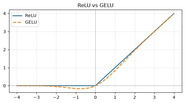

z = torch.linspace(-4, 4, 401)
plt.figure(figsize=(6, 3.4))
plt.plot(z, F.relu(z), label="ReLU", lw=2); plt.plot(z, F.gelu(z), label="GELU", lw=2, ls="--")
plt.axhline(0, color="grey", lw=0.5); plt.axvline(0, color="grey", lw=0.5)
plt.legend(); plt.grid(alpha=0.3); plt.title("ReLU vs GELU"); plt.tight_layout(); plt.show()
print("at z = -1: ReLU", F.relu(torch.tensor(-1.)).item(), "| GELU", round(F.gelu(torch.tensor(-1.)).item(), 4))

Plot output

Output

at z = -1: ReLU 0.0 | GELU -0.1587

For large positive inputs, the two are almost the same. The difference is near zero: ReLU has a sharp corner and outputs exactly 0 for every negative input, while GELU curves smoothly and lets small negative values through (at −1, ReLU gives 0.0 and GELU gives −0.1587). The smooth shape gives gradients for slightly negative inputs too, which tends to make training a little easier.

Check your understandingCheck yourself

The FFN never lets tokens exchange information. Why can a Transformer still produce contextual representations?

Checkpoint Before you move on from §3

How are feed-forward weights used across positions?

Residual Connections

A residual connection (or skip connection) adds a sub-layer's input to its output: instead of x = f(x), we compute x = x + f(x). The sub-layer only has to learn a change to apply to the vector, not a complete new vector.

This matters for two reasons.

Information is preserved. The original token information flows straight up the stack. Each sub-layer adds to it rather than replacing it. This is the "residual stream" picture from Lesson 6.1.
Gradients have a direct path. During backpropagation, the derivative of x + f(x) with respect to x includes a plain "+1" from the x term. So the gradient can flow from the loss back to the early layers along an uninterrupted highway, however deep the stack, instead of being multiplied through every sub-layer in turn, which, as Lesson 5.4 showed, makes gradients shrink.

Let's measure the second point. We build stacks of 1, 4, 12 and 24 blocks, with and without residual connections, pass a random input through, and measure the size of the gradient that arrives back at the input.

Python 17 lines

def input_gradient(depth, residual, seed=0):    """Measure the input-gradient norm of a controlled block stack, with or without residual additions.    Arguments:        depth: Number of stacked blocks.        residual: Whether to retain the residual additions in this controlled experiment.        seed: Random seed for this experiment.    """    torch.manual_seed(seed)    stack = nn.Sequential(*[Block(64, 4, residual=residual) for _ in range(depth)])    x = torch.randn(4, 16, 64, requires_grad=True)    stack(x).pow(2).mean().backward()    return x.grad.norm().item()print(f"{'blocks':>6} {'with residuals':>15} {'without':>12}")for depth in [1, 4, 12, 24]:    print(f"{depth:>6} {input_gradient(depth, True):>15.2e} {input_gradient(depth, False):>12.2e}")

def input_gradient(depth, residual, seed=0):
    """Measure the input-gradient norm of a controlled block stack, with or without residual additions.

    Arguments:
        depth: Number of stacked blocks.
        residual: Whether to retain the residual additions in this controlled experiment.
        seed: Random seed for this experiment.
    """
    torch.manual_seed(seed)
    stack = nn.Sequential(*[Block(64, 4, residual=residual) for _ in range(depth)])
    x = torch.randn(4, 16, 64, requires_grad=True)
    stack(x).pow(2).mean().backward()
    return x.grad.norm().item()

print(f"{'blocks':>6} {'with residuals':>15} {'without':>12}")
for depth in [1, 4, 12, 24]:
    print(f"{depth:>6} {input_gradient(depth, True):>15.2e} {input_gradient(depth, False):>12.2e}")

Output

blocks  with residuals      without
     1        3.33e-02     4.37e-03
     4        4.40e-02     5.11e-03
    12        1.03e-01     5.31e-03
    24        1.54e-01     5.26e-03

With residual connections, the gradient reaching the input is 3.33e-02 for one block and grows to 1.54e-01 for 24 blocks. Without them, it is much smaller at every depth, between 4.37e-03 and 5.31e-03, about 8 times smaller with one block and about 29 times smaller with 24. The deeper the stack, the more the residual path matters. In Section 7 we will see what this means for actual training.

Key terms

Residual (skip) connection: adding a layer's input to its output, x + f(x).

Residual stream: the sequence of token vectors that flows up through the model and that each sub-layer adds to.

Check your understandingCheck yourself

If a sub-layer learns to output all zeros, what does a block with residual connections do to its input?

Checkpoint Before you move on from §4

Why do residual additions help optimisation?

Layer Normalisation

As a vector flows up through many blocks, each adding something to it, its numbers can drift to very different sizes. Large values make later layers behave erratically, and they make the best learning rate hard to choose. Layer normalisation (LayerNorm) keeps every token's vector at a standard scale.

For each token separately, LayerNorm:

computes the mean and variance of that token's numbers;
subtracts the mean and divides by the square root of the variance (plus a tiny number, 1e-5, to avoid dividing by zero), so the vector has mean 0 and standard deviation 1;
multiplies by a learnable scale and adds a learnable shift, so the model can choose a different scale if that helps.

Let's do it by hand for a 4-number vector:

Python 8 lines

v = torch.tensor([2.0, -1.0, 4.0, 3.0])mean, var = v.mean(), v.var(unbiased=False)by_hand = (v - mean) / torch.sqrt(var + 1e-5)ln = nn.LayerNorm(4)print("vector:", v.tolist(), "| mean", mean.item(), "| variance", var.item())print("normalised by hand:", [round(t, 4) for t in by_hand.tolist()])print("nn.LayerNorm:      ", [round(t, 4) for t in ln(v).tolist()])print("learnable scale and shift start at:", ln.weight.tolist(), ln.bias.tolist())

v = torch.tensor([2.0, -1.0, 4.0, 3.0])
mean, var = v.mean(), v.var(unbiased=False)
by_hand = (v - mean) / torch.sqrt(var + 1e-5)
ln = nn.LayerNorm(4)
print("vector:", v.tolist(), "| mean", mean.item(), "| variance", var.item())
print("normalised by hand:", [round(t, 4) for t in by_hand.tolist()])
print("nn.LayerNorm:      ", [round(t, 4) for t in ln(v).tolist()])
print("learnable scale and shift start at:", ln.weight.tolist(), ln.bias.tolist())

Output

vector: [2.0, -1.0, 4.0, 3.0] | mean 2.0 | variance 3.5
normalised by hand: [0.0, -1.6036, 1.069, 0.5345]
nn.LayerNorm:       [0.0, -1.6036, 1.069, 0.5345]
learnable scale and shift start at: [1.0, 1.0, 1.0, 1.0] [0.0, 0.0, 0.0, 0.0]

The vector [2, −1, 4, 3] has mean 2.0 and variance 3.5. Subtracting the mean and dividing by √3.5 gives [0.0, −1.6036, 1.069, 0.5345], exactly what nn.LayerNorm returns. The learnable scale starts at 1 and the shift at 0, so at the start of training LayerNorm is pure standardisation.

Here is its effect on tokens of wildly different sizes:

Python 6 lines

torch.manual_seed(0)xs = torch.randn(2, 5, 64) * torch.tensor([0.1, 1.0, 10.0, 100.0, 1000.0]).view(1, 5, 1)out = nn.LayerNorm(64)(xs)print("std of each token's 64 numbers before:", [round(t, 2) for t in xs[0].std(-1, unbiased=False).tolist()])print("std of each token's 64 numbers after: ", [round(t, 2) for t in out[0].std(-1, unbiased=False).tolist()])print("mean of each token after:              ", [round(abs(t), 4) for t in out[0].mean(-1).tolist()])

torch.manual_seed(0)
xs = torch.randn(2, 5, 64) * torch.tensor([0.1, 1.0, 10.0, 100.0, 1000.0]).view(1, 5, 1)
out = nn.LayerNorm(64)(xs)
print("std of each token's 64 numbers before:", [round(t, 2) for t in xs[0].std(-1, unbiased=False).tolist()])
print("std of each token's 64 numbers after: ", [round(t, 2) for t in out[0].std(-1, unbiased=False).tolist()])
print("mean of each token after:              ", [round(abs(t), 4) for t in out[0].mean(-1).tolist()])

Output

std of each token's 64 numbers before: [0.1, 1.03, 7.91, 85.4, 853.7]
std of each token's 64 numbers after:  [1.0, 1.0, 1.0, 1.0, 1.0]
mean of each token after:               [0.0, 0.0, 0.0, 0.0, 0.0]

Before normalisation, the five tokens' standard deviations range from 0.1 to 853.7. After it, every token has a standard deviation of 1.0 and a mean of 0.0. At initialisation this gives a predictable scale. After training, the learned per-coordinate scale and shift can change the output mean and standard deviation; they need not remain exactly 0 and 1.

Note what LayerNorm normalises over: the 64 numbers within one token. It does not mix information between tokens or between examples in a batch, unlike the batch normalisation used in many CNNs. So it behaves identically in training and inference, and for any batch size.

Key terms

Layer normalisation: rescaling each token's vector to mean 0 and standard deviation 1, followed by a learnable scale and shift.

Check your understandingCheck yourself

LayerNorm is applied to a token vector whose 64 numbers are all equal to 5. What problem arises, and how does the small constant 1e-5 help?

Visual walkthrough: Normalise one token, coordinate by coordinate.

Follow centring, scaling and the learned affine transformation. The coordinates remain different.

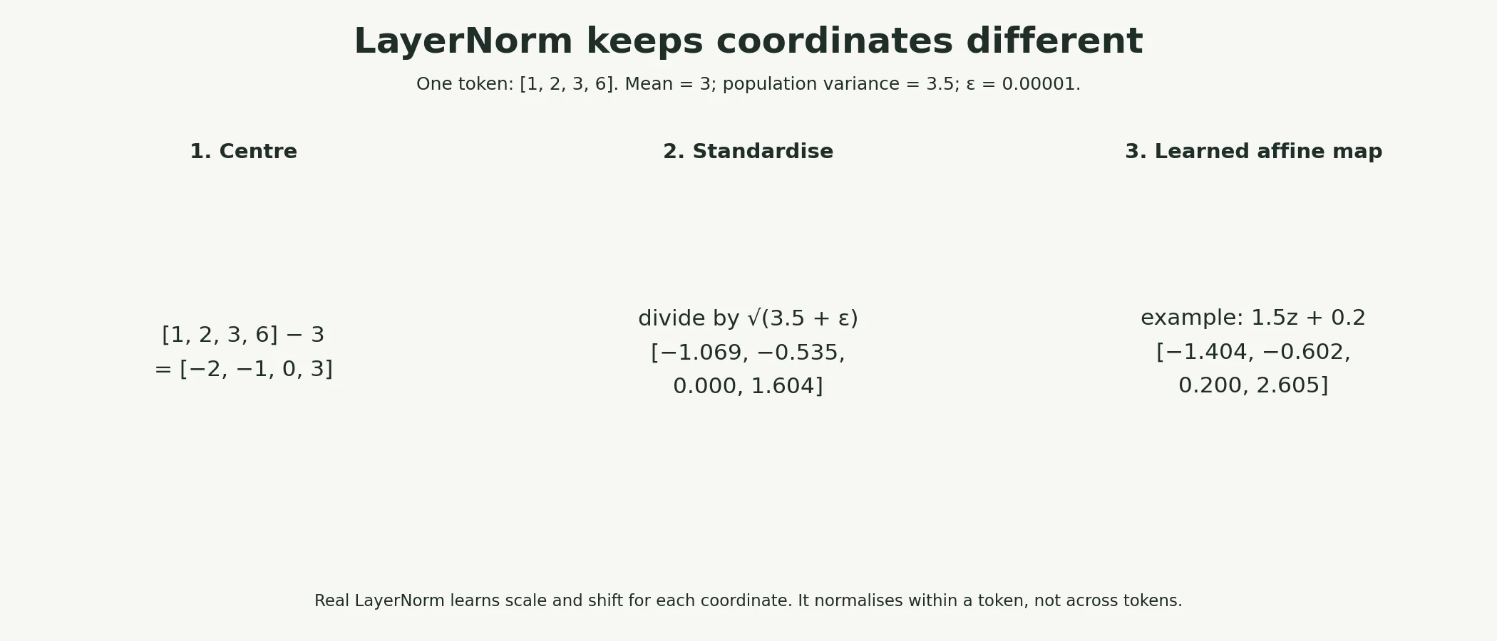
Normalise one token, coordinate by coordinate: a numerical worked example.

These supplied numbers illustrate the calculation. The web app adds a paused, step-by-step animation of the same example.

Checkpoint Before you move on from §5

What does LayerNorm normalise in this model?

The Order of Operations Within a Transformer Block

There are two ways to combine normalisation with the residual connections.

Post-norm (the original Transformer): transform, add, then normalise: x = LayerNorm(x + sublayer(x)). The normalisation sits on the residual stream itself.
Pre-norm (most modern Transformers): normalise the sub-layer's input, transform, then add: x = x + sublayer(LayerNorm(x)). The residual stream is never normalised; it is a clean highway from bottom to top.

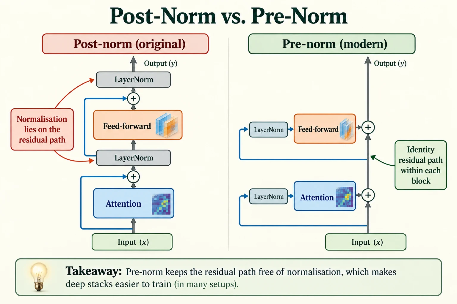
Post-Norm vs. Pre-Norm. Post-norm puts normalisation on the residual path after each addition.

Figure 6.4.2. Post-norm puts normalisation on the residual path after each addition. Pre-norm puts it at each branch input, leaving an identity route within the block. A final model-level norm may still follow the stack; training behaviour depends on the full setup.

The difference looks cosmetic. Let's find out whether it is. We train a 6-block language model on Tiny Shakespeare, predicting the next character, with a fairly high learning rate of 0.01, for 250 steps, in three versions, each with two random seeds:

post-norm, with no warmup;
pre-norm, with no warmup;
post-norm, with a 100-step learning-rate warmup: the learning rate starts near zero and rises linearly to 0.01 over the first 100 steps.

The training function also records the gradient norm at every step: the overall size of all the gradients combined, a useful health check.

Python 61 lines

PATH = "data/shakespeare/input.txt"os.makedirs("data/shakespeare", exist_ok=True)if not os.path.exists(PATH):    urllib.request.urlretrieve("https://raw.githubusercontent.com/karpathy/char-rnn/master/data/tinyshakespeare/input.txt", PATH)text = open(PATH, encoding="utf-8").read()chars = sorted(set(text)); stoi = {c: i for i, c in enumerate(chars)}data = torch.tensor([stoi[c] for c in text]); train_ids = data[:int(0.9 * len(data))]V, D, H, T, B = len(chars), 64, 4, 32, 32class TinyLM(nn.Module):    """Small language model used in the norm-placement and residual-connection experiments."""    def __init__(self, n_layers, pre_norm, residual=True):        """Create the components of this model; the forward computation is traced in the lesson.        Arguments:            n_layers: Number of Transformer blocks.            pre_norm: Whether to normalise sub-layer inputs before their residual additions.            residual: Whether to retain the residual additions in this controlled experiment.        """        super().__init__()        self.tok, self.pos = nn.Embedding(V, D), nn.Embedding(T, D)        self.blocks = nn.Sequential(*[Block(D, H, pre_norm=pre_norm, residual=residual) for _ in range(n_layers)])        self.ln_f = nn.LayerNorm(D) if pre_norm else nn.Identity()   # post-norm blocks already end with a norm        self.head = nn.Linear(D, V)    def forward(self, ids):        """Small language model used in the norm-placement and residual-connection experiments.        Arguments:            ids: Integer token IDs, usually shaped (batch, tokens).        """        return self.head(self.ln_f(self.blocks(self.tok(ids) + self.pos(torch.arange(ids.shape[1])))))def train_run(pre_norm, lr, warmup, steps=250, n_layers=6, seed=0, residual=True):    """Run the specified block-stability experiment and return training losses and measured gradient norms.    Arguments:        pre_norm: Whether to normalise sub-layer inputs before their residual additions.        lr: Learning rate.        warmup: Number of initial learning-rate warmup steps.        steps: Number of optimiser updates.        n_layers: Number of Transformer blocks.        seed: Random seed for this experiment.        residual: Whether to retain the residual additions in this controlled experiment.    """    torch.manual_seed(seed)    model = TinyLM(n_layers, pre_norm, residual)    opt = torch.optim.AdamW(model.parameters(), lr=lr)    g = torch.Generator().manual_seed(seed)    losses, grad_norms = [], []    for step in range(steps):        scale = min(1.0, (step + 1) / warmup) if warmup else 1.0      # linear warmup        for group in opt.param_groups: group["lr"] = lr * scale        starts = torch.randint(0, len(train_ids) - T - 1, (B,), generator=g)        x = torch.stack([train_ids[s:s + T] for s in starts]); y = torch.stack([train_ids[s + 1:s + T + 1] for s in starts])        loss = F.cross_entropy(model(x).view(-1, V), y.view(-1))        opt.zero_grad(); loss.backward()        grad_norms.append(torch.nn.utils.clip_grad_norm_(model.parameters(), float("inf")).item())   # measure only        opt.step(); losses.append(loss.item())    return losses, grad_normsprint("model parameters (6 blocks):", count(TinyLM(6, True)))

PATH = "data/shakespeare/input.txt"
os.makedirs("data/shakespeare", exist_ok=True)
if not os.path.exists(PATH):
    urllib.request.urlretrieve("https://raw.githubusercontent.com/karpathy/char-rnn/master/data/tinyshakespeare/input.txt", PATH)
text = open(PATH, encoding="utf-8").read()
chars = sorted(set(text)); stoi = {c: i for i, c in enumerate(chars)}
data = torch.tensor([stoi[c] for c in text]); train_ids = data[:int(0.9 * len(data))]
V, D, H, T, B = len(chars), 64, 4, 32, 32

class TinyLM(nn.Module):
    """Small language model used in the norm-placement and residual-connection experiments."""
    def __init__(self, n_layers, pre_norm, residual=True):
        """Create the components of this model; the forward computation is traced in the lesson.

        Arguments:
            n_layers: Number of Transformer blocks.
            pre_norm: Whether to normalise sub-layer inputs before their residual additions.
            residual: Whether to retain the residual additions in this controlled experiment.
        """
        super().__init__()
        self.tok, self.pos = nn.Embedding(V, D), nn.Embedding(T, D)
        self.blocks = nn.Sequential(*[Block(D, H, pre_norm=pre_norm, residual=residual) for _ in range(n_layers)])
        self.ln_f = nn.LayerNorm(D) if pre_norm else nn.Identity()   # post-norm blocks already end with a norm
        self.head = nn.Linear(D, V)
    def forward(self, ids):
        """Small language model used in the norm-placement and residual-connection experiments.

        Arguments:
            ids: Integer token IDs, usually shaped (batch, tokens).
        """
        return self.head(self.ln_f(self.blocks(self.tok(ids) + self.pos(torch.arange(ids.shape[1])))))

def train_run(pre_norm, lr, warmup, steps=250, n_layers=6, seed=0, residual=True):
    """Run the specified block-stability experiment and return training losses and measured gradient norms.

    Arguments:
        pre_norm: Whether to normalise sub-layer inputs before their residual additions.
        lr: Learning rate.
        warmup: Number of initial learning-rate warmup steps.
        steps: Number of optimiser updates.
        n_layers: Number of Transformer blocks.
        seed: Random seed for this experiment.
        residual: Whether to retain the residual additions in this controlled experiment.
    """
    torch.manual_seed(seed)
    model = TinyLM(n_layers, pre_norm, residual)
    opt = torch.optim.AdamW(model.parameters(), lr=lr)
    g = torch.Generator().manual_seed(seed)
    losses, grad_norms = [], []
    for step in range(steps):
        scale = min(1.0, (step + 1) / warmup) if warmup else 1.0      # linear warmup
        for group in opt.param_groups: group["lr"] = lr * scale
        starts = torch.randint(0, len(train_ids) - T - 1, (B,), generator=g)
        x = torch.stack([train_ids[s:s + T] for s in starts]); y = torch.stack([train_ids[s + 1:s + T + 1] for s in starts])
        loss = F.cross_entropy(model(x).view(-1, V), y.view(-1))
        opt.zero_grad(); loss.backward()
        grad_norms.append(torch.nn.utils.clip_grad_norm_(model.parameters(), float("inf")).item())   # measure only
        opt.step(); losses.append(loss.item())
    return losses, grad_norms

print("model parameters (6 blocks):", count(TinyLM(6, True)))

Output

model parameters (6 blocks): 310465

Python 6 lines

runs = {}for name, pre, warm in [("post-norm, no warmup", False, 0), ("pre-norm, no warmup", True, 0), ("post-norm, 100-step warmup", False, 100)]:    for seed in [0, 1]:        losses, gn = train_run(pre, lr=1e-2, warmup=warm, seed=seed)        runs[(name, seed)] = (losses, gn)        print(f"{name:<27} seed {seed}: loss over last 25 steps {np.mean(losses[-25:]):.3f} | largest gradient norm {max(gn):.1f}")

runs = {}
for name, pre, warm in [("post-norm, no warmup", False, 0), ("pre-norm, no warmup", True, 0), ("post-norm, 100-step warmup", False, 100)]:
    for seed in [0, 1]:
        losses, gn = train_run(pre, lr=1e-2, warmup=warm, seed=seed)
        runs[(name, seed)] = (losses, gn)
        print(f"{name:<27} seed {seed}: loss over last 25 steps {np.mean(losses[-25:]):.3f} | largest gradient norm {max(gn):.1f}")

Output

post-norm, no warmup        seed 0: loss over last 25 steps 3.341 | largest gradient norm 4.2
post-norm, no warmup        seed 1: loss over last 25 steps 3.317 | largest gradient norm 117.6
pre-norm, no warmup         seed 0: loss over last 25 steps 2.133 | largest gradient norm 1.3
pre-norm, no warmup         seed 1: loss over last 25 steps 2.146 | largest gradient norm 1.1
post-norm, 100-step warmup  seed 0: loss over last 25 steps 2.229 | largest gradient norm 1.4
post-norm, 100-step warmup  seed 1: loss over last 25 steps 2.232 | largest gradient norm 1.6

The results split sharply.

Post-norm, no warmup fails on both seeds: its loss is stuck at 3.341 and 3.317. With seed 1, its gradient norm spiked to 117.6 at one point.
Pre-norm, no warmup trains well on both seeds: 2.133 and 2.146.
Post-norm with warmup trains on both seeds too, 2.229 and 2.232, although a little behind pre-norm after the same number of steps.

What does a loss of about 3.3 mean? Let's compute two reference points:

Python 4 lines

counts = torch.bincount(train_ids, minlength=V).float(); p = counts / counts.sum()unigram = -(p * p.log()).sum().item()print(f"loss of always predicting overall character frequencies: {unigram:.3f}")print(f"loss of a uniform guess, ln({V}): {math.log(V):.3f}")

counts = torch.bincount(train_ids, minlength=V).float(); p = counts / counts.sum()
unigram = -(p * p.log()).sum().item()
print(f"loss of always predicting overall character frequencies: {unigram:.3f}")
print(f"loss of a uniform guess, ln({V}): {math.log(V):.3f}")

Output

loss of always predicting overall character frequencies: 3.309
loss of a uniform guess, ln(65): 4.174

A model that ignores the input and always predicts the overall frequency of each character (how often e, space, t and so on appear) gets a loss of 3.309. A completely uniform guess gets ln(65) = 4.174. The failed post-norm runs, at 3.317 and 3.341, have collapsed to the character-frequency baseline: the model has learned how common each character is, and nothing else. The plot shows it happening.

Python 8 lines

plt.figure(figsize=(7, 4))smooth = lambda a: np.convolve(a, np.ones(10) / 10, mode="valid")for name, c in [("post-norm, no warmup", "tab:red"), ("pre-norm, no warmup", "tab:blue"), ("post-norm, 100-step warmup", "tab:green")]:    plt.plot(smooth(runs[(name, 0)][0]), color=c, label=name)plt.axhline(unigram, color="grey", ls="--", lw=1, label="character-frequency baseline")plt.xlabel("training step"); plt.ylabel("training loss (10-step average)")plt.title("6 blocks, learning rate 0.01, seed 0"); plt.grid(alpha=0.3); plt.legend(fontsize=8)plt.tight_layout(); plt.show()

plt.figure(figsize=(7, 4))
smooth = lambda a: np.convolve(a, np.ones(10) / 10, mode="valid")
for name, c in [("post-norm, no warmup", "tab:red"), ("pre-norm, no warmup", "tab:blue"), ("post-norm, 100-step warmup", "tab:green")]:
    plt.plot(smooth(runs[(name, 0)][0]), color=c, label=name)
plt.axhline(unigram, color="grey", ls="--", lw=1, label="character-frequency baseline")
plt.xlabel("training step"); plt.ylabel("training loss (10-step average)")
plt.title("6 blocks, learning rate 0.01, seed 0"); plt.grid(alpha=0.3); plt.legend(fontsize=8)
plt.tight_layout(); plt.show()

Plot output

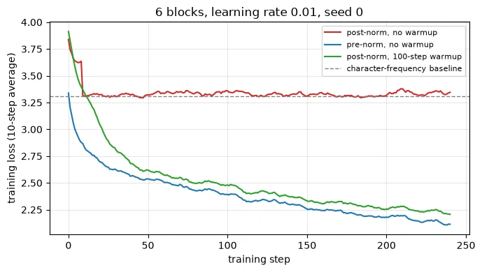
The post-norm run (red) drops quickly, then falls onto the dashed baseline within about ten steps and never leaves it. The pre-norm run (blue) and the warmed-up post-norm run (green) keep improving throughout.

Why does post-norm break? In post-norm, every gradient travelling down the residual stream must pass through a LayerNorm in every block, and early in training, with random weights and a large learning rate, the first updates can be large enough to knock the model into a state from which it does not recover. Warmup avoids those damaging first steps by keeping the early updates small, and pre-norm avoided this failure in our experiment by keeping the residual path free of normalisation.

This is why almost every modern Transformer uses pre-norm, and why warmup is standard practice whenever post-norm (or any fragile setup) is used. The original Transformer paper also trained with a learning-rate warmup.

Common mistake: concluding that a model or dataset "doesn't work" because a loss curve flattens at a baseline. A loss stuck at the character-frequency (or class-frequency) baseline usually means training has collapsed, often because of an unstable setup. Before changing anything else, compare against simple baselines, then try a lower learning rate, warmup or pre-norm.

Key terms

Post-norm / pre-norm: layer normalisation applied after the residual addition / to each sub-layer's input.

Learning-rate warmup: gradually increasing the learning rate from near zero at the start of training.

Gradient norm: the overall size of all gradients combined; a sudden spike is a warning sign.

Training collapse: training that gets stuck at a trivial solution, such as predicting only class frequencies.

Check your understandingCheck yourself

A colleague's post-norm Transformer is stuck at a loss equal to the character-frequency baseline. Suggest two changes, each supported by the experiment above.

Checkpoint Before you move on from §6

What does the pre-norm versus post-norm experiment support?

Stacking Transformer Blocks: Why Depth and Residual Connections Matter

A single block lets each token gather information once and process it once. Stacking blocks lets the model build on what earlier blocks found. One block might connect each character to the one before it; a later block can then use that to recognise whole words; later still, which speaker is talking. Each block's attention works on vectors that already contain context from the blocks below, so the reach and complexity of what the model can represent grows with depth: the same hierarchy idea as CNN layers in Lesson 5.2.

Depth costs parameters, but each block adds the same amount:

Python 3 lines

for d in [1, 3, 6, 12, 24]:    m = TinyLM(d, True)    print(f"{d:>2} blocks: {count(m):>9,} parameters")

for d in [1, 3, 6, 12, 24]:
    m = TinyLM(d, True)
    print(f"{d:>2} blocks: {count(m):>9,} parameters")

Output

 1 blocks:    60,545 parameters
 3 blocks:   160,513 parameters
 6 blocks:   310,465 parameters
12 blocks:   610,369 parameters
24 blocks: 1,210,177 parameters

Each extra block adds 49,984 parameters (for example, 60,545 for one block, 160,513 for three and 310,465 for six; the rest is the embeddings, final norm and output head). Large language models stack dozens of much wider blocks.

But depth only helps if the stack can be trained. In Section 4 we saw that removing residual connections makes the gradient reaching the input much smaller. Here is what that means in practice: the same 6-block pre-norm model, trained for 200 steps at a learning rate of 0.003, with and without residual connections.

Python 4 lines

for residual in [True, False]:    losses, _ = train_run(True, lr=3e-3, warmup=0, steps=200, n_layers=6, residual=residual)    print(f"6 pre-norm blocks, {'with' if residual else 'WITHOUT'} residual connections: "          f"loss over last 25 steps {np.mean(losses[-25:]):.3f}")

for residual in [True, False]:
    losses, _ = train_run(True, lr=3e-3, warmup=0, steps=200, n_layers=6, residual=residual)
    print(f"6 pre-norm blocks, {'with' if residual else 'WITHOUT'} residual connections: "
          f"loss over last 25 steps {np.mean(losses[-25:]):.3f}")

Output

6 pre-norm blocks, with residual connections: loss over last 25 steps 2.267
6 pre-norm blocks, WITHOUT residual connections: loss over last 25 steps 3.296

With residual connections, the model reaches a loss of 2.267. Without them, it reaches 3.296: almost exactly the character-frequency baseline of 3.309. Without the residual highway, this 6-block model learns essentially nothing about context in 200 steps. This experiment shows how important residual connections are for this deep stack and training budget; it does not prove that every non-residual architecture is untrainable.

Check your understandingCheck yourself

Why might a 1-block model without residual connections still train reasonably, while a 6-block model without them fails?

Checkpoint Before you move on from §7

Why can depth add useful computation?

Putting It All Together

A Transformer block takes (batch, tokens, d_model) and returns the same shape, through two sub-layers:

x = x + attention(layer_norm_1(x))
x = x + feed_forward(layer_norm_2(x))

Attention (16,640 parameters in our block) gathers information between tokens. The feed-forward network (33,088 parameters) processes each token separately, expanding to 256 numbers, applying GELU and contracting again. Residual connections add each sub-layer's output to its input, preserving information and giving gradients a direct path: without them, the gradient reaching the input was about 29 times smaller in a 24-block stack, and a 6-block model got stuck at 3.296, the character-frequency baseline. Layer normalisation rescales each token to mean 0 and standard deviation 1, whatever its size was before.

The order of these ingredients matters. At a learning rate of 0.01, post-norm blocks collapsed to the baseline on both seeds (3.341 and 3.317), while pre-norm blocks trained (2.133 and 2.146), and a 100-step warmup rescued post-norm (2.229 and 2.232). That is why our model, like most modern ones, uses pre-norm.

Stacking blocks adds 49,984 parameters each and lets later blocks build on what earlier ones found. In Lesson 6.5 we stack three of them into a complete language model.

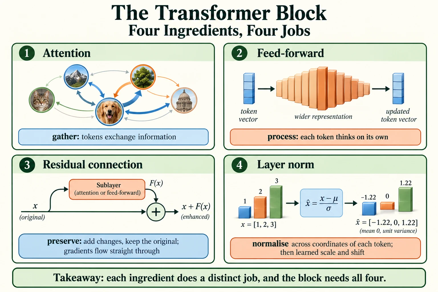
Four Ingredients, Four Jobs. Attention gathers across allowed positions, the feed-forward network transforms each position, residual addition preserves a direct path, and LayerNorm standardises coordinates within each token before learned scale and shift.

Figure 6.4.3. Attention gathers across allowed positions, the feed-forward network transforms each position, residual addition preserves a direct path, and LayerNorm standardises coordinates within each token before learned scale and shift. LayerNorm does not make coordinates equal.

Summary

A Transformer block has two sub-layers, attention and feed-forward, each with layer normalisation and a residual connection. Its input and output shapes are the same.
Attention gathers information between tokens; the feed-forward network processes each token separately (64 → 256 → 64 with GELU) and holds most of the block's parameters.
Residual connections (x + f(x)) preserve information and give gradients a direct path; without them, gradients reaching the input were far smaller and a 6-block model failed to learn (3.296 vs. 2.267).
Layer normalisation rescales each token's vector to mean 0 and standard deviation 1, with a learnable scale and shift.
Pre-norm (normalise each sub-layer's input) trains reliably; post-norm collapsed at a high learning rate unless the learning rate was warmed up.
A loss stuck at the character-frequency baseline (3.309 here) is a sign of training collapse.
Stacking blocks adds 49,984 parameters each and lets later blocks build on earlier ones.

Glossary

Term	Meaning
Transformer block	Attention and feed-forward sub-layers, each with layer norm and a residual connection.
Sub-layer	One of the two parts of a block: attention or feed-forward.
Feed-forward network (FFN)	A two-layer MLP applied to each token separately.
GELU	A smooth activation function similar to ReLU, used in most modern Transformers.
Residual (skip) connection	Adding a sub-layer's input to its output: `x + f(x)`.
Residual stream	The token vectors flowing up the model, which each sub-layer adds to.
Layer normalisation	Rescaling each token's vector to mean 0 and standard deviation 1, plus a learnable scale and shift.
Post-norm	Normalising after the residual addition (original Transformer).
Pre-norm	Normalising each sub-layer's input (modern Transformers).
Learning-rate warmup	Raising the learning rate gradually at the start of training.
Gradient norm	The overall size of all gradients combined.
Training collapse	Training stuck at a trivial solution, such as predicting only frequencies.
Character-frequency baseline	The loss of always predicting each character's overall frequency.

Wrap-up

Knowledge check

Why keep a block's input and output shapes equal?

Why do residual additions help optimisation?

Why can depth add useful computation?

Questions and discussion

Ask about this lesson, share what you found in a lab, or help someone else. Posts are public on the course's GitHub Discussions: anyone can read them, and you need a GitHub account to post.

Opening it loads giscus from giscus.app.

Before you start

Prerequisites

The Big Picture: How a Transformer Block Works

Multi-Head Self-Attention

Feed-Forward Networks

Residual Connections

Layer Normalisation

Normalise one token, coordinate by coordinate

The Order of Operations Within a Transformer Block

Stacking Transformer Blocks: Why Depth and Residual Connections Matter

Putting It All Together

Summary

Glossary

Wrap-up

Quick check

Questions and discussion