When Gradients Misbehave
- Time
- ~65 min
- Sections
- 8
- Code cells
- 13
- Labs
- 3
- Figures
- 4
Before you start
A falling loss does not prove every layer is learning. You turn Module 2's single gradient norm into a per-layer probe and use it to catch five failures: a broken initialisation (all zeros, or far too large), vanishing gradients through a deep sigmoid stack (nine orders of magnitude between first and last layer), exploding gradients and what clipping does about them, dead ReLU units behind Lesson 3.1's collapse, and the two structural fixes, normalisation and residual connections. The lesson ends with a layer-health checklist you can run on any model.
- Learning goal
Lessons 3.1 and 3.2 mostly treated the model as one object: you changed a setting, trained it, and read the loss or validation metric. That is useful, but it can hide an important class of failures.
A neural network is a chain of layers, and each layer learns only through the gradient that reaches it. If the gradient reaching one layer is extremely small, that layer may barely change even while the overall loss is improving. If the gradient is extremely large, one update can throw the weights into a bad numerical state. Neither problem is necessarily obvious from the loss curve alone.
This notebook therefore moves the diagnostic inside the network. You will measure the gradient received by each layer, deliberately create several ways for gradient flow to fail, and then connect each failure to a specific intervention.
By the end, the goal is not to memorise a collection of fixes. It is to look at a broken training run and ask: which part of the computation is failing, what evidence would reveal it, and which mechanism explains that evidence?
- You will be able to
- Turn the single gradient-norm probe from Module 2 into a reusable per-layer diagnostic
- Explain why weight initialisation affects whether a network can learn effectively at all
- Measure vanishing gradients and explain how the chain rule and saturating activations cause them
- Measure exploding gradients and understand what gradient clipping actually changes
- Detect dead ReLU units and connect them to the learning-rate collapse from Lesson 3.1
- Explain what BatchNorm and LayerNorm normalise, how they affect gradient flow, and why their use differs
- Explain why a residual connection creates a direct route for gradients
- Apply a compact layer-health checklist to an unfamiliar model
A per-layer gradient probe
In Module 2, Lesson 2.3 §9 you computed one gradient norm after loss.backward(). That number is useful as a quick check that some gradient exists, but it combines information from all parameters.
That combination can hide the problem we care about. Imagine the first layer has gradient norm 1e-10 while the last layer has gradient norm 1.0. The total can still look perfectly ordinary because the large gradient from the last layer dominates the summary.
So we need a more informative measurement: the gradient norm for each layer separately.
The important idea is simple:
loss.backward()computes how much the loss would change if each parameter changed.p.gradstores that gradient for parameterp.- The norm, such as
p.grad.norm(), gives one number describing the overall size of that parameter's gradient. - Looking at those numbers from the first layer to the last lets us see whether the learning signal is reaching every part of the network.
We are not measuring whether a layer is "good" in isolation. We are measuring whether the backward signal reaching different depths is on a comparable scale.
def layer_grad_norms(model, xb, yb, loss_function=None): """Run one forward/backward pass and return the gradient norm of each weight matrix. The Module 2 gradient-norm probe, computed per layer instead of summed. The model is put in training mode, gradients are cleared before and after, and only 2-D parameters (weight matrices) are reported, in forward order. Args: model: The network to probe. xb: A batch of inputs. yb: The matching targets, shaped like the model's output. loss_function: Loss taking ``(output, target)``; defaults to the global ``loss_fn``. Returns: A list of ``(parameter_name, gradient_norm)`` pairs, first layer first. """ loss_function = loss_function or loss_fn model.train() model.zero_grad() loss = loss_function(model(xb), yb) loss.backward() out = [] for name, p in model.named_parameters(): if p.grad is not None and p.dim() > 1: # weight matrices only, skip biases out.append((name, p.grad.norm().item())) model.zero_grad() return outdef summarise(tag, norms): """Print the first, middle and last gradient norms of a profile and their ratio. Args: tag: Label printed at the start of the line. norms: A list of ``(name, norm)`` pairs from ``layer_grad_norms``. Returns: The ratio last-layer norm ÷ first-layer norm (huge = vanishing). """ first, last = norms[0][1], norms[-1][1] ratio = last / max(first, 1e-30) print(f"{tag:<22} first {first:.3e} mid {norms[len(norms)//2][1]:.3e} " f"last {last:.3e} last/first {ratio:.3e}") return ratiodef plot_profiles(profiles, title): """Plot one or more per-layer gradient profiles on a log scale. Args: profiles: Dict mapping a label to a list of ``(name, norm)`` pairs. title: Title of the figure. """ plt.figure(figsize=(9, 4.2)) for tag, norms in profiles.items(): plt.plot(range(1, len(norms)+1), [n for _, n in norms], "o-", ms=4, lw=1.7, label=tag) plt.yscale("log"); plt.xlabel("layer (1 = closest to input)") plt.ylabel("gradient norm (log scale)"); plt.title(title) plt.legend(fontsize=9); plt.grid(alpha=0.3, which="both") plt.tight_layout(); plt.show()# sanity check on a shallow, healthy networktorch.manual_seed(SEED)shallow = nn.Sequential(nn.Linear(D,64), nn.ReLU(), nn.Linear(64,32), nn.ReLU(), nn.Linear(32,1))for n, g in layer_grad_norms(shallow, Xt[:256], Yt[:256]): print(f" {n:<12} grad norm {g:.4e}")One forward and backward pass, then one gradient norm per weight matrix, in forward order.
- 1
Training mode, so BatchNorm uses batch statistics as it would during a real training step.
- 2
2-D tensors are the weight matrices; biases and normalisation parameters (1-D) are skipped.
- 3
p.grad.norm()is the Frobenius norm: the square root of the sum of every squared gradient element. - 4
Returned as well as printed. When
summariseis the last line of a cell, Jupyter also echoes this number.
  0.weight     grad norm 1.1257e-01
  2.weight     grad norm 1.5730e-01
  4.weight     grad norm 1.4339e-01
On a shallow, healthy network, the gradient norms of the layers are usually in roughly the same order of magnitude. That does not mean they must be identical. It means there is no enormous systematic gap where one part of the network receives a useful learning signal and another receives almost none.
Think of this function as an instrument rather than as part of the model. We will use it throughout the notebook to answer a specific diagnostic question:
Where in the network is the learning signal becoming too small or too large?
Lesson 3.4 will eventually connect this probe to the config-driven runner from Module 2 so that the same measurement can be recorded automatically during experiments.
A network's summed gradient norm looks perfectly normal. What can it still hide?
A large last-layer gradient dominates the total. Per-layer norms show where the learning signal is lost or amplified.
What question does the per-layer gradient probe answer, and what does a 'healthy' profile look like?
- It asks where in the network the learning signal becomes too small or too large, layer by layer.
- Healthy: layers' gradient norms are within roughly the same order of magnitude, with no huge systematic gap between early and late layers.
Initialisation is not a detail
Before training begins, every trainable weight needs an initial numerical value. Initialisation is the rule used to choose those starting values.
It is tempting to regard this as a minor implementation detail because the optimizer will change the weights anyway. But the starting values determine the scale of the first activations and gradients, and they can also determine whether different hidden units begin with different behaviour.
We will compare three schemes while keeping the architecture and training procedure fixed:
- sensible framework-style initialisation;
- all-zero weights;
- deliberately enormous weights.
The point is not to memorise one magic initialisation formula. The point is to understand what a broken initialisation looks like and why it breaks.
def build_with_init(kind, seed=SEED): """Build the 3-layer ReLU MLP (61 → 64 → 32 → 1) with a chosen initialisation. Args: kind: ``"default"`` (PyTorch's own initialisation), ``"zeros"`` (every weight and bias 0), ``"big"`` (weights drawn with standard deviation 3, biases 0) or ``"kaiming"`` (Kaiming-normal weights for ReLU, biases 0). seed: Seed for the random initialisation. Returns: The initialised ``nn.Sequential``. """ torch.manual_seed(seed) m = nn.Sequential(nn.Linear(D,64), nn.ReLU(), nn.Linear(64,32), nn.ReLU(), nn.Linear(32,1)) if kind == "default": return m # PyTorch's own initialisation for mod in m: if isinstance(mod, nn.Linear): if kind == "zeros": nn.init.zeros_(mod.weight); nn.init.zeros_(mod.bias) elif kind == "big": nn.init.normal_(mod.weight, 0.0, 3.0); nn.init.zeros_(mod.bias) elif kind == "kaiming": nn.init.kaiming_normal_(mod.weight, nonlinearity="relu"); nn.init.zeros_(mod.bias) return mdef short_train(model, epochs=8, lr=1e-3, bs=32, seed=SEED): """Train a model briefly with AdamW and report its losses and validation AUC. Args: model: The model to train (modified in place). epochs: Number of passes over the 500 training rows. lr: Learning rate. bs: Mini-batch size. seed: Seed for the batch order. Returns: A tuple ``(losses, auc)``: the mean training loss of each epoch and the validation ROC-AUC after training. """ opt = torch.optim.AdamW(model.parameters(), lr=lr) g = torch.Generator().manual_seed(seed) dl = torch.utils.data.DataLoader(torch.utils.data.TensorDataset(Xt, Yt), batch_size=bs, shuffle=True, generator=g) losses = [] for ep in range(epochs): model.train(); tot = n = 0 for xb, yb in dl: opt.zero_grad(); l = loss_fn(model(xb), yb); l.backward(); opt.step() tot += l.item()*len(xb); n += len(xb) losses.append(tot/n) model.eval() with torch.no_grad(): auc = roc_auc_score(y_va, torch.sigmoid(model(Xv)).numpy().ravel()) return losses, aucfor kind in ["zeros", "big", "kaiming", "default"]: m = build_with_init(kind) losses, auc = short_train(m) print(f"{kind:<9} epoch losses {' '.join(f'{x:9.4f}' for x in losses[:4])} ... val AUC {auc:.4f}")- 1
nn.Lineardraws weights and biases uniformly from ±1/√fan_in. - 2
Everything zero: no hidden weight will ever receive a gradient (see the explainer below).
- 3
Standard deviation 3, about 40 times the default for 61 inputs (1/√(3·61) ≈ 0.074).
- 4
Standard deviation √(2/fan_in): the scale that keeps a ReLU layer's signal size roughly constant.
zeros     epoch losses    0.6918    0.6889    0.6860    0.6832 ...   val AUC 0.5000
big       epoch losses  641.5191  548.8349  483.1462  448.8655 ...   val AUC 0.5329
kaiming   epoch losses    0.6495    0.5829    0.5435    0.5150 ...   val AUC 0.8153
default   epoch losses    0.6975    0.6317    0.5880    0.5700 ...   val AUC 0.8133
# Why zeros fails: check whether the hidden units differ from each other at all.m0 = build_with_init("zeros")_ = short_train(m0, epochs=3)W1 = m0[0].weight.detach()print("after 3 epochs of training from an all-zeros init:")print(f" layer-1 weight matrix shape {tuple(W1.shape)}")print(f" number of DISTINCT rows (hidden units): {len(torch.unique(W1, dim=0))}")print(f" std across the 64 hidden units: {W1.std(dim=0).mean().item():.3e}")print()print("Every hidden unit received the same gradient and made the same update,")print("so all 64 units are identical. The layer has the expressive power of ONE unit.")print()mb = build_with_init("big")print("Why a too-large init fails:")with torch.no_grad(): h = mb[0](Xt[:256])print(f" pre-activation std at layer 1: {h.std().item():.2f} (healthy is around 1)")print(f" fraction of activations killed by ReLU: {(mb[1](h) == 0).float().mean().item():.1%}")after 3 epochs of training from an all-zeros init: layer-1 weight matrix shape (64, 61) number of DISTINCT rows (hidden units): 1 std across the 64 hidden units: 0.000e+00 Every hidden unit received the same gradient and made the same update, so all 64 units are identical. The layer has the expressive power of ONE unit. Why a too-large init fails: pre-activation std at layer 1: 12.76 (healthy is around 1) fraction of activations killed by ReLU: 50.7%
Deep diveWhat actually happened in the all-zeros run
With every weight and bias at zero, each hidden activation is ReLU(0) = 0 for every row, so the output is just the last layer's
bias. The backward signal to a layer passes through the next layer's weights, which are zero, so no hidden weight ever receives a
gradient: the 64 units are not only identical, they never move. The only parameter that learns is the output bias, which drifts
towards the base rate. That is why the loss creeps down (0.692, 0.689, 0.686, …, heading for the 30% base-rate loss of 0.611) while the
AUC stays at exactly 0.5: a constant prediction ranks nobody.
Two different failures appear here, and they have different mechanisms.
All zeros: the symmetry problem
If every weight in a layer starts at exactly the same value, the hidden units start in exactly the same state. They therefore produce the same activations, receive the same gradients, and make the same updates. Nothing distinguishes one unit from another, so they remain identical.
This is called symmetry. A 64-unit layer may contain 64 parameter sets, but if all those units behave identically, the network is not getting 64 independent pieces of representation.
Random initialisation is therefore not mainly about adding randomness for its own sake. Its important job is to break symmetry, giving different units slightly different starting points so they can specialise.
Very large weights: the scale problem
With a standard deviation of 3.0, the initial weights are deliberately far too large. That produces very large pre-activations and a huge starting loss. For ReLU networks, many units can also be pushed into the negative region, where ReLU outputs zero and has zero derivative.
The network is no longer failing because its units are identical. It is failing because the numerical scale of the computation is badly behaved.
What sensible initialisation is trying to preserve
Kaiming-style initialisation chooses the scale of weights using the number of inputs to a layer. The aim is to keep the variance of activations from changing wildly as the signal moves forward through the network.
PyTorch's standard Linear initialisation is already designed to give sensible starting scales, so you usually do not need to hand-design initialisation for ordinary layers.
What you do need to recognise are the signatures of a broken start:
- a loss that begins at an absurdly large value;
- a metric that remains at chance;
- gradients that are essentially zero;
- or activations that immediately become numerically extreme.
With the Default initialisation, find the largest learning rate that still reaches 95% test accuracy with no more than 6 dead units in layer 1 after 25 epochs.
-
If all weights are zero but the biases are non-zero, why does the symmetry problem remain? And if every weight is instead set to the same non-zero value such as
0.1, what has changed — and what has not?Zero weights, non-zero biases. Each hidden unit's output is then a function of its bias alone: it does not depend on the input at all. The backward signal to a layer also has to pass through the next layer's weights, which are zero, so at first the early layers receive no gradient. When updates do start to reach the first layer, every unit's update is the same input direction scaled by a different number, so all 64 rows of the weight matrix point the same way and the layer effectively learns one feature. With equal biases the units stay exactly identical; with different biases they only get different offsets along that single direction. Random weights are what give each unit its own direction from the start.
Every weight 0.1. The signal now flows: activations depend on the input and gradients are non-zero, so the network learns. But every unit in a layer still has the same weights (and biases), so they compute the same value, receive the same gradient and make the same update, forever. The symmetry is unchanged: each layer behaves like a single unit, however wide it is.
Why does an all-zero weight initialisation fail?
After training, the 64-unit layer had one distinct row. Random initialisation's main job is to break symmetry.
Weights initialised with standard deviation 3.0 gave a starting loss of about 640. What is the failure mechanism?
Different mechanism from zeros: the units differ, but the computation's scale is extreme. Kaiming-style (and PyTorch default) init keeps activation variance stable.
If all weights are the same non-zero value, say 0.1, has the symmetry problem been fixed? Explain.
- No. Every unit in the layer still computes the same function, receives the same gradient and makes the same update, so they stay identical.
- Only the starting scale changed; breaking symmetry needs different (random) starting values per unit. (Non-zero biases that are all equal do not help either.)
Vanishing gradients
Now we reach a failure that becomes much more important as a network gets deeper.
Backpropagation uses the chain rule. To find how the loss changes with respect to an early layer, the gradient is passed backward through every operation between that layer and the loss. In simplified form, those local derivatives are multiplied together.
That creates a simple numerical effect:
- if many factors are smaller than
1, their product becomes very small; - if many factors are larger than
1, their product can become very large.
For example, multiplying by 0.3 twelve times gives roughly 5e-7. The exact network is more complicated than this toy calculation, but the principle is the same.
The sigmoid activation makes the first case especially visible. Its derivative is never larger than 0.25, and it becomes much smaller when the sigmoid is saturated near 0 or 1.
Let's measure what happens as the gradient travels through a deep network.
An untrained 12-layer sigmoid network, one backward pass. How much smaller is the gradient reaching the first layer than the one reaching the last?
About six billion times (1.9e-10 against 1.1). The 12-layer ReLU network loses a factor of about 4,500: much better, still far from healthy. The lab below lets you rebuild both and see where the signal goes.
def deep_net(activation="sigmoid", n_layers=12, width=64, norm=None, seed=0): """Build a deep MLP for studying gradient flow. ``n_layers`` weight matrices in total: an input layer, ``n_layers − 2`` hidden ``width × width`` layers (each optionally followed by LayerNorm or BatchNorm) and an output layer, with the chosen activation after every layer but the last. Args: activation: ``"sigmoid"``, or anything else for ReLU. n_layers: Total number of linear layers. width: Width of every hidden layer. norm: ``None``, ``"ln"`` for LayerNorm or ``"bn"`` for BatchNorm1d, applied after each hidden linear layer. seed: Seed for the initial weights. Returns: An ``nn.Sequential`` producing one logit per row. """ torch.manual_seed(seed) Act = nn.Sigmoid if activation == "sigmoid" else nn.ReLU layers = [nn.Linear(D, width), Act()] for _ in range(n_layers - 2): layers.append(nn.Linear(width, width)) if norm == "ln": layers.append(nn.LayerNorm(width)) if norm == "bn": layers.append(nn.BatchNorm1d(width)) layers.append(Act()) layers.append(nn.Linear(width, 1)) return nn.Sequential(*layers)profiles = {}xb, yb = Xt[:256], Yt[:256]for tag, act in [("12-layer sigmoid", "sigmoid"), ("12-layer ReLU", "relu")]: norms = layer_grad_norms(deep_net(act), xb, yb) profiles[tag] = norms summarise(tag, norms)print()print("For reference, the 3-layer healthy network:")summarise("3-layer ReLU", layer_grad_norms(build_with_init("default"), xb, yb))- 1
This is the cell's last expression, so Jupyter displays
summarise's return value: the stray1.2737…below is the healthy network's last/first ratio.
12-layer sigmoid       first 1.859e-10   mid 5.458e-05   last 1.111e+00   last/first 5.977e+09
12-layer ReLU          first 2.421e-05   mid 1.066e-03   last 1.100e-01   last/first 4.545e+03

For reference, the 3-layer healthy network:
3-layer ReLU           first 1.126e-01   mid 1.573e-01   last 1.434e-01   last/first 1.274e+00
1.2737144876680562
plot_profiles(profiles, "Gradient norm by depth — the signal dies on the way down")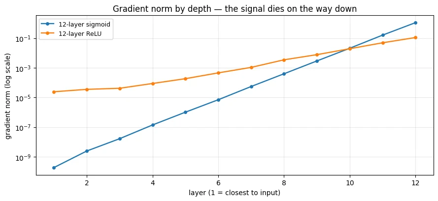
The numbers are stark. In the 12-layer sigmoid network, the gradient reaching the first layer is roughly nine orders of magnitude smaller than the gradient reaching the last layer.
What does that mean in practice?
The layers near the output are receiving a usable learning signal. The layers near the input are receiving such a tiny signal that their weights may barely change at all. The network can therefore reduce the loss while a large portion of its depth contributes very little learning.
This is an important diagnostic lesson: a falling loss does not prove that every layer is training properly.
ReLU improves the situation because its derivative is 1 whenever its input is positive. In that active region, ReLU itself does not shrink the gradient. That is one major reason ReLU became a standard hidden activation instead of sigmoid.
But ReLU alone does not guarantee healthy gradient flow. In a deep network, the product of the linear-layer derivatives can still create a large difference between early and late layers. Sections 6 and 7 introduce two structural tools that address this more directly: normalisation and residual connections.
The same chain-rule issue also helps explain why very deep recurrent networks historically had difficulty learning long-range dependencies. An RNN unrolled over many time steps creates a long sequence of transformations through which the gradient must travel. LSTMs introduced gating mechanisms that provided additional ways for information and gradients to persist. Attention takes a different route by allowing positions to interact without requiring every dependency to pass through one long sequential chain.
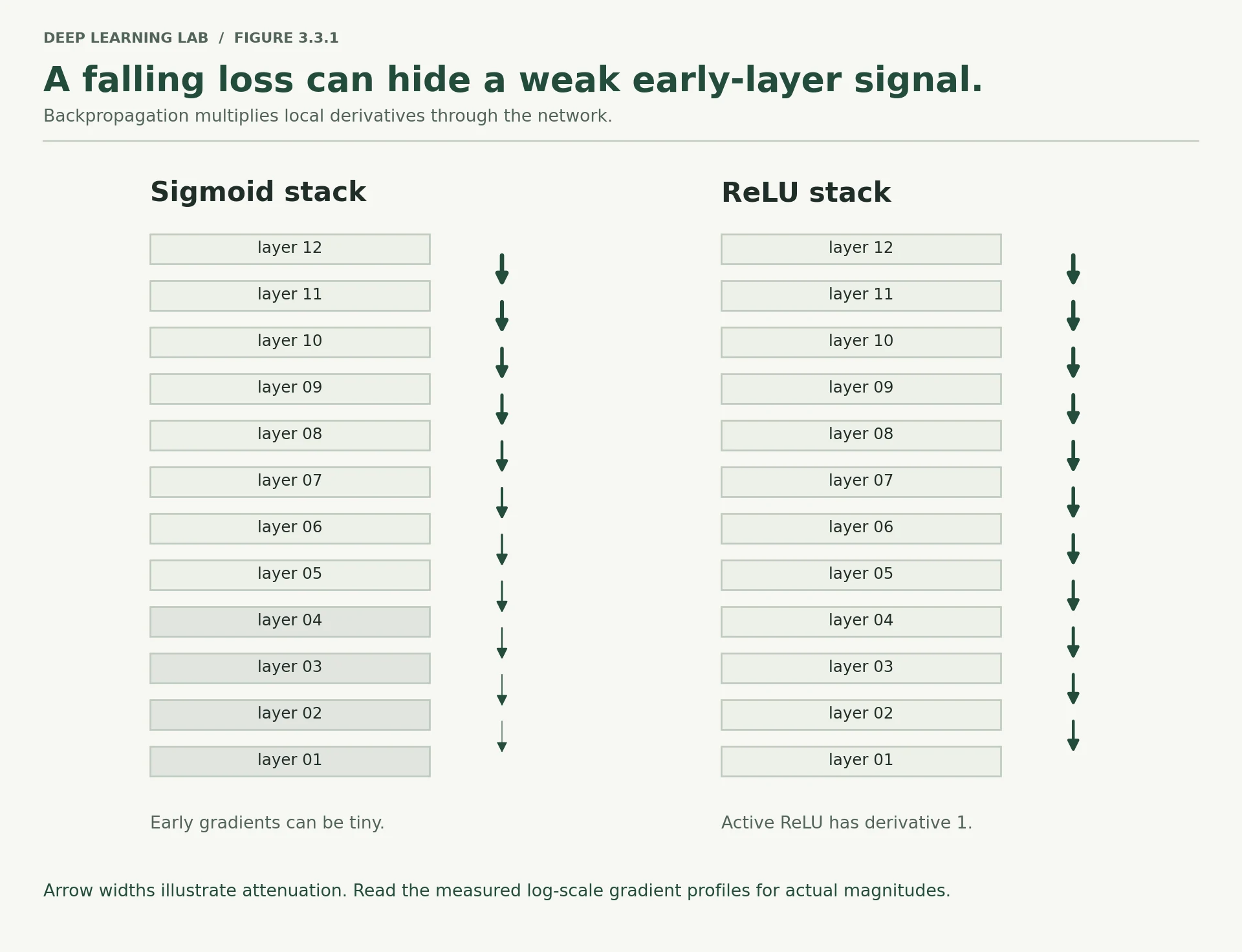
Synthetic inputs, so the exact numbers differ from the notebook's, but the orders of magnitude match: sigmoid about 1e10, ReLU about 5e3, LayerNorm, BatchNorm and residual all within about 10.
-
The profile above was measured on an untrained network, immediately after initialisation. Would you expect the sigmoid network's gradient profile to become healthier or worse after many training steps? Explain your reasoning in terms of saturation: what happens to the sigmoid derivative when its inputs become very positive or very negative?
Usually worse. Training tends to make weights larger, and larger weights push pre-activations further from zero. Once an input to a sigmoid is far from zero the sigmoid saturates: its output sits near 0 or 1 and its slope \(\sigma(z)(1-\sigma(z))\) falls from 0.25 towards zero (0.0066 at \(z = 5\)). Each saturated layer multiplies the backward signal by that tiny slope, so the early layers, which were already receiving about a billionth of the last layer's gradient, receive even less. The later layers keep learning, which makes the network more confident and the saturation worse. This self-reinforcing effect is why deep sigmoid networks were so hard to train, and why ReLU, normalisation and residual connections replaced them.
What is the largest slope the sigmoid function can have?
\(\sigma'(z) = \sigma(z)(1-\sigma(z)) \le 0.25\), reached at \(z = 0\). Twelve such factors shrink a gradient enormously.
In the 12-layer sigmoid network, the first layer's gradient was about \(10^{9}\) times smaller than the last's. What does that mean in practice?
A falling loss does not prove every layer is training. ReLU helps (slope 1 when active) but does not guarantee healthy flow in deep stacks.
Would the sigmoid network's gradient profile get better or worse as training pushes activations to extremes? Explain with 'saturation'.
- Worse. When sigmoid inputs become very positive or very negative, the output saturates near 1 or 0 and the derivative approaches 0.
- Saturated layers pass back even smaller factors, so the vanishing gets stronger.
Exploding gradients, and clipping
The same chain-rule mechanism can fail in the opposite direction.
If the factors being multiplied through the backward pass are repeatedly greater than 1, the product grows rapidly with depth. The result is an exploding gradient: an unusually large gradient reaches some parameters, producing an unusually large parameter update.
A common symptom is a training run that appears normal and then suddenly:
- the loss jumps to an enormous value;
- the loss becomes
NaNorInf; - activations or weights become numerically extreme;
- or the next few updates are completely unusable.
The important point is that one oversized update can be enough to destabilise the rest of training.
Gradient clipping is a direct way to limit that update. The next experiment shows what it does and, just as importantly, what it does not do.
explode = deep_net("relu", n_layers=12)for mod in explode: if isinstance(mod, nn.Linear): nn.init.normal_(mod.weight, 0.0, 1.5) # deliberately too largeexplode.train(); explode.zero_grad()loss_fn(explode(xb), yb).backward()total = torch.sqrt(sum(p.grad.pow(2).sum() for p in explode.parameters())).item()print(f"total gradient norm with a 1.5-sigma init: {total:.3e}")print()lr = 1e-3with torch.no_grad(): biggest = max(p.grad.abs().max().item() for p in explode.parameters())print(f"largest single gradient element: {biggest:.3e}")print(f"at lr={lr}, that one weight would move by {lr*biggest:.3e} in a single step")print(" (a typical healthy weight has magnitude around 0.1)")total gradient norm with a 1.5-sigma init: 4.306e+10 largest single gradient element: 8.832e+09 at lr=0.001, that one weight would move by 8.832e+06 in a single step (a typical healthy weight has magnitude around 0.1)
# Gradient clipping: rescale the whole gradient if its norm exceeds a threshold.explode2 = deep_net("relu", n_layers=12)for mod in explode2: if isinstance(mod, nn.Linear): nn.init.normal_(mod.weight, 0.0, 1.5)explode2.train(); explode2.zero_grad()loss_fn(explode2(xb), yb).backward()before = nn.utils.clip_grad_norm_(explode2.parameters(), max_norm=1.0) # returns the PRE-clip normafter = torch.sqrt(sum(p.grad.pow(2).sum() for p in explode2.parameters())).item()print(f"norm before clipping: {before.item():.3e}")print(f"norm after clipping : {after:.4f}")print()print("Where it goes in the training loop:")print(" loss.backward()")print(" nn.utils.clip_grad_norm_(model.parameters(), max_norm=1.0) # <- between")print(" optimizer.step()")print()print("Clipping preserves the DIRECTION of the gradient and caps only its LENGTH.")- 1
Clips in place and returns the norm before clipping: log it during training to see how often clipping fires.
- 2
The same total norm, recomputed by hand: exactly
max_normafter clipping.
norm before clipping: 4.306e+10
norm after clipping : 1.0000

Where it goes in the training loop:
    loss.backward()
    nn.utils.clip_grad_norm_(model.parameters(), max_norm=1.0)   # <- between
    optimizer.step()

Clipping preserves the DIRECTION of the gradient and caps only its LENGTH.
Gradient clipping rescales the gradient when its norm is larger than a chosen threshold.
Suppose the gradient vector has norm 10 and the threshold is 1. Clipping scales the whole vector down so that its norm becomes 1. The direction stays the same; only the magnitude changes.
That gives clipping a very specific role: it prevents a single update from being catastrophically large. It does not discover why the gradient became large in the first place.
The placement is important enough to memorise:
backward() → clip gradients → step()
Clipping before backward() would not clip the gradients produced by the current loss. Clipping after step() would be too late because the oversized parameter update has already happened.
A threshold such as 1.0 is a common starting point, but there is no universal threshold that is correct for every model. The right lesson is not "always use 1.0." It is:
Use clipping as protection against unusually large updates, then investigate the cause if clipping is happening constantly.
If gradients repeatedly hit the clipping threshold, possible causes include poor initialisation, an excessive learning rate, or badly scaled inputs. Continually lowering the threshold can hide the symptom without fixing the underlying problem.
Two ways to clip
clip_grad_norm_(params, max_norm)Rescales all gradients together when their combined norm exceeds max_norm. Direction preserved. The usual choice.
clip_grad_value_(params, clip_value)Clamps each element to ±clip_value separately. Large components are cut more than small ones, so the direction changes.
Choose a learning rate and max_norm so the clipped path reaches the minimum in 6 steps or fewer.
Implement clip_grad_norm_
Given a list of gradient arrays, compute their total norm (as if they were one long vector). If it exceeds max_norm, scale every
array by max_norm / total. Return the clipped list and the total norm before clipping.
Where does gradient clipping go in the training loop?
Before backward there is nothing to clip; after step the oversized update has already happened.
What does clip_grad_norm_(params, max_norm=1.0) change?
It prevents one catastrophic update. It does not fix the cause.
Clipping fires on almost every step of your run. What should you do, and what should you not do?
- Investigate the cause: learning rate too high, poor initialisation or badly scaled inputs.
- Don't just keep lowering the threshold: that hides the symptom without fixing the problem.
Dead ReLU units
ReLU is defined as max(0, x).
That simple definition gives it a useful property: for positive inputs, its derivative is 1, so active units do not shrink the gradient. But it also creates a hard failure mode.
For negative inputs, ReLU outputs exactly 0, and its derivative is 0. If a hidden unit ends up producing negative pre-activations for every training example, that unit receives no useful gradient from those examples. It can become permanently inactive — a dead ReLU.
This is different from ordinary overfitting or poor performance. The problem is local: a particular unit has effectively stopped participating in learning.
Lesson 3.1 gave us a suspected cause: the very large learning rate that caused the model to collapse to a constant prediction. Here we will measure whether dead units are the mechanism behind that collapse.
Train the same model at learning rate 0.5. What share of the first layer's ReLU units end up dead (zero on every training row)?
60.9%. At 0.01 it is 12.5% and the model is fine; at 0.5 most of the layer is gone and validation AUC falls to 0.5000. The Unit health lab in §2 lets you watch it happen.
def dead_fraction(model, X, layer_idx=1): """Fraction of units in a ReLU layer that output 0 for every row of ``X``. Runs ``model[0]`` (the first linear layer) and then ``model[layer_idx]`` on the data in evaluation mode, so it is meant for the first activation of a sequential model. Args: model: An ``nn.Sequential`` whose first module is a linear layer. X: Input rows to check. layer_idx: Index of the activation module to apply after ``model[0]``. Returns: The fraction of units (0 to 1) whose largest output over all rows is 0. """ model.eval() with torch.no_grad(): acts = model[layer_idx](model[0](X)) return (acts.max(dim=0).values == 0).float().mean().item()print(f"{'learning rate':>14}{'dead layer-1 units':>22}{'val AUC':>10}")print("-" * 46)for lr in [1e-3, 1e-2, 1e-1, 0.5, 2.0]: torch.manual_seed(SEED) m = nn.Sequential(nn.Linear(D,64), nn.ReLU(), nn.Linear(64,32), nn.ReLU(), nn.Linear(32,1)) opt = torch.optim.AdamW(m.parameters(), lr=lr) g = torch.Generator().manual_seed(SEED) dl = torch.utils.data.DataLoader(torch.utils.data.TensorDataset(Xt, Yt), batch_size=32, shuffle=True, generator=g) for _ in range(5): m.train() for xb_, yb_ in dl: opt.zero_grad(); loss_fn(m(xb_), yb_).backward(); opt.step() m.eval() with torch.no_grad(): auc = roc_auc_score(y_va, torch.sigmoid(m(Xv)).numpy().ravel()) print(f"{lr:>14}{dead_fraction(m, Xt):>21.1%}{auc:>10.4f}")- 1
Run only the first linear layer and its ReLU on every row.
- 2
A unit is dead if its largest output over all rows is 0: it never fires on this data.
 learning rate    dead layer-1 units   val AUC
----------------------------------------------
         0.001                 0.0%    0.7808
          0.01                12.5%    0.7955
           0.1                43.8%    0.7367
           0.5                60.9%    0.5000
           2.0                60.9%    0.5000
There is the causal chain that Lesson 3.1 could only suggest.
A learning rate that is too large can move the first-layer weights so far in one update that many ReLU units are pushed permanently into their zero-output region. Once a unit is dead, its gradient is zero, so later updates cannot bring it back. If enough units die, the layer loses most of its useful representation capacity and the whole model can collapse toward a constant prediction — hence AUC near 0.5.
But do not turn this into the rule "any dead ReLU is bad." A modest fraction of inactive units can be completely harmless. Neural networks are often over-parameterised, so the surviving units can carry the useful computation.
What matters is the fraction of a layer that has become inactive and whether that loss of capacity is associated with degraded model behaviour.
This failure is permanent for the current training run. Lowering the learning rate after the units have died does not give them a gradient to recover with. In practice, you normally restart training after fixing the cause.
Useful responses include:
- Lower the learning rate when large updates are the cause.
- Use LeakyReLU or GELU when you want a non-zero gradient on the negative side.
- Check input scaling. Features with very different or very large scales can create extreme pre-activations and gradients. The
StandardScalerin this pipeline is therefore part of the numerical-stability story, not merely cosmetic preprocessing.
The measurement is simple enough to keep in your diagnostic toolkit: ask what fraction of units in a layer never activate on the data being inspected.
-
The function above tests whether a unit is inactive for every training row. Could a unit be active somewhere in the training set but inactive for every validation row? If so, what might that tell you about the relationship between the training and validation feature distributions?
Yes. A unit can fire only for a few training rows, for example rows with a rare category or an extreme numeric value, and for none of the 250 validation rows. On the training set it counts as alive; on validation it contributes nothing.
Two readings are possible. With a small validation set it can simply mean the region of feature space that unit responds to is rare and happened to be missing from the validation sample. If many units behave this way, it suggests the network has built units for a handful of specific training rows (a sign of memorisation), or that validation data differs from training data in which regions of the feature space it covers (a distribution shift). Comparing each unit's firing rate on training and validation is a cheap way to find out which.
Most of a layer's ReLU units are dead after training at lr = 0.5. Lowering the learning rate now…
A unit inactive for every row receives no gradient. Remedies: a smaller learning rate, LeakyReLU/GELU, and scaled inputs, then restart.
Is any dead ReLU unit a problem?
Networks are over-parameterised. At lr = 0.5, 61% died and AUC fell to 0.5; at lr = 0.01, 12.5% died and AUC was fine.
Normalisation as a stabiliser
The previous sections showed two opposite gradient problems: gradients can become extremely small or extremely large as they pass through depth.
A useful way to understand both is to focus on scale. If the activations entering each layer become progressively too large or too small, the local derivatives in the chain rule can also become badly scaled. That makes the product through many layers unstable.
Normalisation layers try to control that scale by rescaling activations during the forward pass.
The two normalisation schemes we need to distinguish are based on different sets of values:
- BatchNorm normalises each feature using statistics computed across the examples in the current batch. For a particular feature, it asks: "How are the values for this feature distributed across these rows?"
- LayerNorm normalises each individual example across its features. For one row, it asks: "How are this example's feature activations distributed?"
So the difference is not simply two names for the same operation. They use different axes and therefore have different behaviour with respect to batch size and evaluation mode.
Let's measure how these choices affect gradient flow.
norm_profiles = {}for tag, kw in [("no norm", dict(norm=None)), ("LayerNorm", dict(norm="ln")), ("BatchNorm", dict(norm="bn"))]: norms = layer_grad_norms(deep_net("relu", n_layers=12, **kw), xb, yb) norm_profiles[tag] = norms summarise(f"12-layer ReLU, {tag}", norms)12-layer ReLU, no norm first 2.421e-05 mid 1.066e-03 last 1.100e-01 last/first 4.545e+03 12-layer ReLU, LayerNorm first 1.571e-01 mid 8.388e-01 last 1.149e+00 last/first 7.313e+00 12-layer ReLU, BatchNorm first 1.154e+00 mid 3.651e-01 last 8.440e-01 last/first 7.316e-01
plot_profiles(norm_profiles, "Normalisation flattens the gradient profile across depth")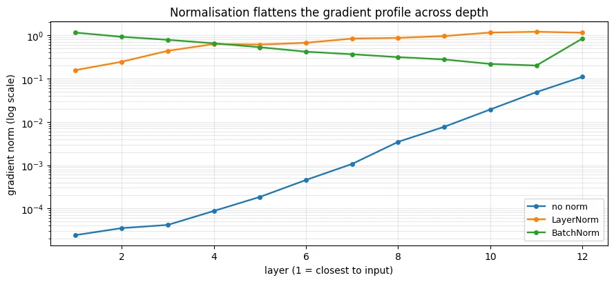
This experiment shows the structural effect clearly. In the plain 12-layer ReLU network, the gradient reaching the last layer can be thousands of times larger than the gradient reaching the first. Adding LayerNorm reduces that gap to single digits, while BatchNorm brings it close to one in this particular experiment.
The important lesson is not that BatchNorm will always beat LayerNorm numerically. The lesson is that normalisation can keep the scale of intermediate activations and gradients under control, making deep stacks easier to train.
BatchNorm
BatchNorm computes statistics across examples in a batch. That creates a dependency between rows: during training, the representation of one row is partly determined by the other rows that happen to be in the same batch.
That can work very well, particularly in convolutional vision models, but it becomes less convenient with very small or variable batches.
It also explains why model.train() and model.eval() matter. During training, BatchNorm uses batch statistics and updates running statistics. During evaluation, it uses the stored running statistics instead of recomputing them from the evaluation batch.
LayerNorm
LayerNorm normalises each example independently across its features. There is therefore no dependence on the other rows in the batch.
That property is particularly useful for sequence models and Transformers, where batch composition should not determine how an individual sequence is normalised. LayerNorm is consequently a standard component of Transformer architectures.
You do not need to derive the backward pass here. What you should be able to explain is what is being normalised, over which dimensions, and why that choice matters.
BatchNorm and LayerNorm, side by side
Mean and variance of each feature across the rows of the batch. Training uses the batch's statistics and updates running averages; eval() uses the running averages. Needs batches bigger than one row. Typical in vision CNNs.
Mean and variance of each row across its 64 features. Identical in training and evaluation, independent of batch size and of the other rows. Standard in Transformers.
-
Why is it acceptable for BatchNorm to use information from other rows during training, but not desirable to recompute those batch statistics independently at inference time? What does PyTorch do differently in
eval()mode?During training the batch statistics are part of a stochastic training procedure, much like dropout or the random order of mini-batches: they normalise activations using the rows at hand, and the small amount of noise they add even acts as a mild regulariser. At inference the requirement is different: a customer's prediction must depend only on that customer. Recomputing statistics from the inference batch would make the same row score differently depending on which other rows it arrived with, would break entirely for a batch of one (the variance of one value is zero), and would drift whenever a batch is unrepresentative.
So in
eval()mode PyTorch's BatchNorm uses the running mean and variance it accumulated during training (an exponential average,momentum=0.1), stops updating them, and normalises every row with those fixed values, which makes evaluation deterministic and independent of batch composition. (In training mode, a batch of one row raises an error for exactly this reason.)
What does model.eval() change for BatchNorm?
Training uses batch statistics (and updates running averages); evaluation uses the running averages, so each row's output does not depend on its batch-mates.
Why is LayerNorm the standard choice in Transformers?
BatchNorm normalises each feature across the batch; LayerNorm normalises each row across its features.
Explain the difference between BatchNorm and LayerNorm by the axis each one normalises over.
- BatchNorm: for each feature, statistics across the examples in the batch, so an example's output depends on the other rows (and on train/eval mode).
- LayerNorm: for each example, statistics across its features, so there is no dependence on the rest of the batch.
Residual connections in one line
Normalisation changes the scale of the signal. A residual connection changes the route the signal takes.
A plain block computes:
y = f(x)
A residual block computes:
y = x + f(x)
The original input x is therefore passed directly to the output as well as through the learned transformation f.
Why does this help gradients?
Differentiate the expression with respect to x:
dy/dx = 1 + f'(x)
The important part is the constant 1. Even if the derivative through f becomes very small, the gradient still has a direct path through the x term.
This is the core idea. You do not need a complicated derivation to remember it:
A residual connection gives the gradient a route that bypasses the transformation.
That route becomes extremely valuable when many blocks are stacked.
The plain 12-layer ReLU network's last/first gradient ratio is about 4,500. Change every block from \(f(x)\) to \(x + f(x)\). The ratio becomes about…
About 9.4, nearly three orders of magnitude better from one change to the block. The identity path gives the gradient a route that bypasses every transformation.
class ResidualBlock(nn.Module): """A residual block: returns ``x + f(x)`` with ``f`` = ``Linear → ReLU``. The identity path adds the input back to the transformed value, which gives the gradient a direct route around ``f``. """ def __init__(self, width=64): """Create the transformation ``f``. Args: width: Size of the input and of the output (they must match to be added). """ super().__init__() self.f = nn.Sequential(nn.Linear(width, width), nn.ReLU()) def forward(self, x): """Apply the block. Args: x: Input of shape ``(N, width)``. Returns: ``x + f(x)``, shape ``(N, width)``. """ return x + self.f(x) # <- the residual connectiondef deep_residual(n_layers=12, width=64, residual=False, seed=0): """Build a deep MLP whose hidden blocks are plain ``f(x)`` or residual ``x + f(x)``. Args: n_layers: Total number of linear layers. width: Width of every hidden layer. residual: Use ``ResidualBlock`` for the hidden blocks instead of plain ``Linear → ReLU``. seed: Seed for the initial weights. Returns: An ``nn.Sequential`` producing one logit per row. """ torch.manual_seed(seed) layers = [nn.Linear(D, width), nn.ReLU()] for _ in range(n_layers - 2): layers.append(ResidualBlock(width) if residual else nn.Sequential(nn.Linear(width, width), nn.ReLU())) layers.append(nn.Linear(width, 1)) return nn.Sequential(*layers)res_profiles = {}for tag, flag in [("plain (12 layers)", False), ("residual (12 layers)", True)]: norms = layer_grad_norms(deep_residual(residual=flag), xb, yb) res_profiles[tag] = norms summarise(tag, norms)- 1
The input is added back to the transformed value, so the gradient reaches
xdirectly as well as throughf.
plain (12 layers)      first 2.421e-05   mid 1.066e-03   last 1.100e-01   last/first 4.545e+03
residual (12 layers)   first 7.441e-01   mid 1.061e+00   last 7.006e+00   last/first 9.416e+00
plot_profiles(res_profiles, "A residual connection gives the gradient a direct route")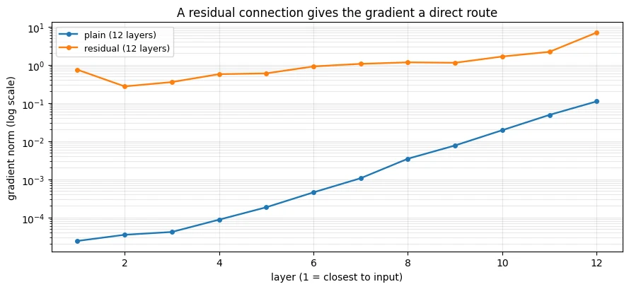
The experiment shows nearly three orders of magnitude of improvement — roughly a factor of 500 — simply by changing the block from f(x) to x + f(x).
The important mechanism is the direct path. In a plain deep network, the gradient must pass through every transformation. In a residual network, part of the gradient can travel along the identity path instead.
This is one reason very deep residual networks can be trained reliably. The problem with adding depth is not only that a larger model can overfit; before residual connections became standard, depth itself could make optimisation difficult because early layers stopped receiving a useful gradient.
There is another useful way to understand residual learning. A residual block does not have to learn the entire desired transformation. It only has to learn the difference from the identity. If leaving the representation unchanged is already close to the right thing, the block can make f(x) close to zero and let the skip path carry the representation through unchanged.
Real residual architectures sometimes change the width of the representation. In that case, x and f(x) cannot be added directly because their shapes differ. A common solution is a learned projection — often a linear layer — on the shortcut path so that the two tensors have matching shapes.
-
If the input has width 64 and the transformed path has width 128, why can you not simply write
x + self.f(x)? What would a projection on the residual path need to accomplish, and would the shortcut still provide a direct gradient route?xhas shape(N, 64)andself.f(x)has shape(N, 128). Element-wise addition needs matching shapes, and broadcasting cannot match 64 with 128, so PyTorch raises a size-mismatch error.A projection on the shortcut must map 64 features to 128, usually with a learned linear layer (a 1×1 convolution in a CNN):
y = P(x) + f(x). It should be cheap and simple, typically a single linear map with no activation, so that it does not become a second deep path.The shortcut still provides a short gradient route: the gradient reaches
xthrough one matrix \(P^\top\) instead of through the whole transformationf, but it is no longer the pure identity. Real architectures therefore use projections only where the width changes and keep identity shortcuts everywhere else.
Why does \(y = x + f(x)\) help gradients reach early layers?
The identity path bypasses the transformation. The 12-layer residual net's last/first ratio fell from ~4,500 to ~9.
A block's input has width 64 but \(f(x)\) has width 128. What do you need?
The shortcut still gives a short, direct path for the gradient, now through one linear map rather than the whole block.
A layer-health checklist
The experiments above are different demonstrations of one underlying idea: a training curve tells you what happened overall; internal diagnostics help explain why.
When an unfamiliar model is behaving strangely, you do not want to immediately change five hyperparameters and hope one helps. Start by measuring the internal state of the computation.
The following checklist packages the measurements from this notebook into a quick first pass.
def layer_health_report(model, X, Y, name="model"): """Run this lesson's diagnostics on a model and print a short report. One forward/backward pass gives the per-layer gradient profile and the total gradient norm; one forward pass counts dead units in the first ReLU (when the model starts with ``Linear`` then ``ReLU``). Flags are raised for vanishing or inverted profiles (ratio above 1e3 or below 1e-3), exploding (total norm above 1e3) or absent gradients (below 1e-6), NaN/Inf, and more than half of the first layer's units being dead. Args: model: The model to inspect (its gradients are cleared afterwards). X: A batch of inputs. Y: The matching targets. name: Label for the report. Returns: The list of flag messages; empty when nothing looks wrong. """ print(f"=== layer health: {name} ===") norms = layer_grad_norms(model, X, Y) first, last = norms[0][1], norms[-1][1] ratio = last / max(first, 1e-30) print(f" layers with weight matrices : {len(norms)}") print(f" gradient norm, first layer : {first:.3e}") print(f" gradient norm, last layer : {last:.3e}") print(f" ratio last/first : {ratio:.3e}") flags = [] if ratio > 1e3: flags.append("VANISHING: early layers receive ~no gradient") if ratio < 1e-3: flags.append("INVERTED: late layers receive ~no gradient") # total gradient norm needs its own backward pass, since layer_grad_norms cleared them model.train(); model.zero_grad() loss_fn(model(X), Y).backward() total = torch.sqrt(sum(p.grad.pow(2).sum() for p in model.parameters() if p.grad is not None)).item() print(f" total gradient norm : {total:.3e}") if total > 1e3: flags.append("EXPLODING: consider clip_grad_norm_") if total < 1e-6: flags.append("NO SIGNAL: total gradient is ~zero") if not np.isfinite(total): flags.append("NaN/Inf in gradients") # dead units in the first activation, if there is one model.eval() with torch.no_grad(): try: acts = model[1](model[0](X)) if isinstance(model[1], nn.ReLU): dead = (acts.max(dim=0).values == 0).float().mean().item() print(f" dead units, first ReLU : {dead:.1%}") if dead > 0.5: flags.append(f"DEAD RELU: {dead:.0%} of first-layer units never fire") except Exception: pass model.zero_grad() print(" " + ("status: no flags raised" if not flags else "FLAGS:")) for f in flags: print(f" - {f}") print() return flagslayer_health_report(build_with_init("default"), xb, yb, "3-layer ReLU, default init")layer_health_report(deep_net("sigmoid", 12), xb, yb, "12-layer sigmoid")layer_health_report(deep_net("relu", 12, norm="bn"), xb, yb, "12-layer ReLU + BatchNorm")bad = deep_net("relu", 12)for mod in bad: if isinstance(mod, nn.Linear): nn.init.normal_(mod.weight, 0.0, 1.5)layer_health_report(bad, xb, yb, "12-layer ReLU, 1.5-sigma init")=== layer health: 3-layer ReLU, default init ===
layers with weight matrices : 3
gradient norm, first layer : 1.126e-01
gradient norm, last layer : 1.434e-01
ratio last/first : 1.274e+00
total gradient norm : 3.787e-01
dead units, first ReLU : 1.6%
status: no flags raised
=== layer health: 12-layer sigmoid ===
layers with weight matrices : 12
gradient norm, first layer : 1.859e-10
gradient norm, last layer : 1.111e+00
ratio last/first : 5.977e+09
total gradient norm : 1.157e+00
FLAGS:
- VANISHING: early layers receive ~no gradient
=== layer health: 12-layer ReLU + BatchNorm ===
layers with weight matrices : 12
gradient norm, first layer : 1.154e+00
gradient norm, last layer : 8.440e-01
ratio last/first : 7.316e-01
total gradient norm : 2.219e+00
dead units, first ReLU : 0.0%
status: no flags raised
=== layer health: 12-layer ReLU, 1.5-sigma init ===
layers with weight matrices : 12
gradient norm, first layer : 4.879e+09
gradient norm, last layer : 1.883e+10
ratio last/first : 3.861e+00
total gradient norm : 4.306e+10
dead units, first ReLU : 0.0%
FLAGS:
- EXPLODING: consider clip_grad_norm_
['EXPLODING: consider clip_grad_norm_']
The checklist, in the order you should run it
- Check the total gradient norm. The absolute value depends on the model and loss, so treat the ranges here as rough warning signs, not laws. A norm above about
1e3can indicate explosion; a value below about1e-6can indicate that the learning signal is effectively disappearing. - Check the per-layer gradient profile. Look for a large systematic gap between early and late layers. A last/first ratio of more than roughly three orders of magnitude is a strong reason to investigate.
- Check the fraction of dead ReLU units. A small inactive fraction can be normal. If roughly half or more of a layer is permanently inactive, most of that layer's capacity has been lost.
- Check explicitly for
NaNandInf. These values can propagate through subsequent calculations and turn a useful numerical computation into nonsense. - Check activation scale. If pre-activation standard deviations are extremely large or extremely small, investigate initialisation, input scaling, learning rate, or normalisation.
These checks are diagnostic signals, not universal pass/fail thresholds. The exact healthy range depends on architecture, parameterisation, batch size, loss, and data. Their value is that they turn a vague statement such as "the model is not learning" into a more specific question such as "the early layers are receiving gradients 10,000 times smaller than the final layer."
What to take away
A summed gradient norm hides structure. Per-layer measurements tell you where the learning signal is being lost or amplified.
Initialisation affects the starting numerical regime. All-zero weights preserve symmetry and prevent hidden units from specialising; excessively large weights can create extreme activations and gradients. Standard PyTorch layers already use sensible defaults, so the skill is recognising broken behaviour rather than memorising a custom initialisation recipe.
Vanishing and exploding gradients have the same mathematical family. Both arise from repeated multiplication through the chain rule. When the factors are effectively below one, gradients shrink; when they are effectively above one, they grow.
Dead ReLU units are a local, potentially permanent failure. A unit that receives zero gradient because it is always in ReLU's inactive region cannot repair itself during that run. Excessive learning rates are one important cause.
Normalisation and residual connections address gradient flow structurally. Normalisation controls activation scale; residual connections provide a shortcut path for information and gradients. These are not arbitrary tricks — each changes a specific part of the computation that was causing the problem.
Transition to Lesson 3.4
You now have three kinds of diagnostic evidence:
- Lesson 3.1: learning-rate and optimisation signatures
- Lesson 3.2: generalisation and overfitting signatures
- Lesson 3.3: gradient-flow and internal-layer signatures
The remaining problem is procedural. When a new experiment fails, which measurement should you make first? And how do you avoid changing settings until something happens and then mistaking the change for a diagnosis?
Lesson 3.4 turns these measurements into a diagnostic protocol ordered by cost and evidence, then gives you six deliberately broken experiments to diagnose — including a case where the usual curves look healthy even though the model is still not useful.
A layer-health report shows a last/first gradient ratio of \(10^4\) and 55% dead units in layer 1. What is the value of the report?
The thresholds are warning signs, not laws. The point is to measure before changing five settings and hoping.
Wrap-up
- Measure gradients per layer: a summed norm lets a healthy last layer hide a first layer that receives almost nothing.
- Initialisation sets the starting regime. All-zero weights keep units identical (here, frozen); weights far too large make activations, losses and gradients explode.
- Backpropagation multiplies one factor per layer: below 1 they vanish, above 1 they explode. Sigmoid (slope ≤ 0.25) vanishes fastest; PyTorch's default init also shrinks deep ReLU stacks, Kaiming init does not.
- Gradient clipping (
backward→clip_grad_norm_→step) caps the length of an update and keeps its direction. If it fires constantly, find the cause. - A ReLU unit that is negative for every row gets no gradient and cannot recover in that run. Too-large learning rates kill them in bulk; restart after fixing the cause.
- Normalisation controls activation scale: BatchNorm across the batch (eval uses running statistics), LayerNorm across each row's features (same in train and eval).
- A residual block
x + f(x)gives the gradient a direct route:d/dx = 1 + f′(x). - Run the layer-health checklist on any unfamiliar model: total gradient norm, per-layer profile, dead units, NaN/Inf, activation scale.
Quick check
A network's summed gradient norm looks normal. What can it still hide?
A first layer at 1e-10 and a last layer at 1 give a total of about 1.
Why does an all-zero initialisation fail?
Random initialisation breaks symmetry. With every weight and bias at zero, only the output bias learns.
What is the largest slope a sigmoid can have?
σ′(z) = σ(z)(1 − σ(z)), at most 0.25 at z = 0, and far smaller when saturated.
Where does gradient clipping go in the training loop?
The gradients must exist to be clipped, and the step must not have happened yet.
Most of a layer's ReLU units are dead after training at lr = 0.5. Lowering the learning rate now:
A unit that outputs 0 for every row has zero gradient, so no learning rate can move it.
What does model.eval() change for BatchNorm?
Predictions must not depend on which other rows share the batch.
Why does y = x + f(x) help gradients reach early layers?
The identity path carries the gradient past the transformation.
Questions and discussion
Ask about this lesson, share what you found in a lab, or help someone else. Posts are public on the course's GitHub Discussions: anyone can read them, and you need a GitHub account to post.
Opening it loads giscus from giscus.app.