Understanding the Transformer Architecture
Classroom material
- Time
- ~34 min
- Sections
- 11
- Code cells
- 12
- Figures
- 5
Before you start
What is a Transformer, as a whole, and how does information flow through it?
- You will be able to
- describe the Transformer as a pipeline from tokens to predictions, naming each stage;
- explain what problem the Transformer was designed to solve;
- explain the roles of token embeddings, positional information, attention, feed-forward networks and the output head;
- distinguish encoder-only, decoder-only and encoder–decoder Transformers, and the masks they use;
- trace the shape of the data through a Transformer, layer by layer.
Module 5 ended with a cliffhanger. In Lesson 5.4 we saw that recurrent networks pass information along a chain, one step at a time, squeezing everything through a fixed-size memory. Then we built a single attention step, in which every position could look directly at every other position, and saw that its learning signal did not fade with distance.
The Transformer is what you get when you build an entire network around that idea. It was introduced in a research paper titled "Attention Is All You Need", originally for machine translation, and it has since become the architecture behind almost every major language model, including the large chat assistants you may have used, as well as many modern image, audio and multimodal models.
This module follows the whole-to-parts approach. In this first note, we look at the Transformer as one complete system: what goes in, what comes out, what each major part is for, and how the different families of Transformer differ. We will build a small working Transformer straight away from PyTorch's ready-made parts, so that you can see the whole machine run before we take it apart. In Lessons 6.2 to 6.5 we examine each part in detail and rebuild it ourselves, and in Lesson 6.6 we train it to write text.
Key question: What is a Transformer, as a whole, and how does information flow through it?
Prerequisites
complete Module 5, especially Lessons 5.3 (embeddings) and 5.4 (from sequences to attention).
Setup — imports, versions and device detection used by the notebook (1 cells)
Run this cell first. This lesson trains nothing; it only builds models and passes data through them, so it runs in seconds.
Environment and results. The saved outputs record one CPU reference run; random seeds reduce variation but do not guarantee identical numbers across computers. Read the comparisons as evidence from that run. Training times depend on your hardware.
If packages are missing, install them into your notebook environment, then restart the kernel and run from the beginning:
%pip install torch==2.14.1 numpy==2.5.4 pandas==3.0.6 matplotlib==3.11.2 scikit-learn==1.9.1 scipy==1.18.1
import os, gzip, math, urllib.requestimport numpy as npimport torchimport torch.nn as nnimport torch.nn.functional as Fimport matplotlib.pyplot as plttorch.manual_seed(0)print("PyTorch", torch.__version__)PyTorch 2.14.1+cu130
The Big Picture: What Is a Transformer?
A Transformer is a network that takes a sequence of tokens and produces a new vector for every token, where each new vector has been enriched with information from the other tokens in the sequence. Stack enough of these enrichment steps, add a final layer that turns vectors into predictions, and you have a model that can classify text, translate it, or generate it one token at a time.
It helps to think of a Transformer as a meeting. Each token arrives with its own notes (its embedding). In each round of the meeting, every token gets to listen to the others, decide who is relevant to it, and update its notes accordingly. That listening is attention. Between rounds, each token also takes a moment to think privately about what it has heard: that is the feed-forward network. After several rounds, each token's notes describe not just itself, but its role in the whole sequence.
Throughout this module, we work with Tiny Shakespeare: about a million characters of Shakespeare's plays in one text file. Our models will read and write it one character at a time, which keeps the vocabulary tiny and lets us train on a CPU.
os.makedirs("data/shakespeare", exist_ok=True)PATH = "data/shakespeare/input.txt"if not os.path.exists(PATH): urllib.request.urlretrieve("https://raw.githubusercontent.com/karpathy/char-rnn/master/data/tinyshakespeare/input.txt", PATH)text = open(PATH, encoding="utf-8").read()chars = sorted(set(text))stoi = {c: i for i, c in enumerate(chars)}itos = {i: c for c, i in stoi.items()}encode = lambda s: [stoi[c] for c in s]decode = lambda ids: "".join(itos[i] for i in ids)print("characters in the file:", len(text), "| distinct characters (vocabulary):", len(chars))print(text[:100])print(encode("First Citizen"))characters in the file: 1115394 | distinct characters (vocabulary): 65 First Citizen: Before we proceed any further, hear me speak. All: Speak, speak. First Citizen: You [18, 47, 56, 57, 58, 1, 15, 47, 58, 47, 64, 43, 52]
The file contains 1,115,394 characters, built from just 65 distinct characters: letters, digits, punctuation, the space and the newline. Each character gets a number, its token ID; "First Citizen" becomes [18, 47, 56, 57, 58, 1, 15, 47, 58, 47, 64, 43, 52]. (We look at tokenisation properly in Lesson 6.2.)
Now here is a complete, working Transformer. We build it from PyTorch's ready-made nn.TransformerEncoderLayer, so it fits in a few lines. Don't worry about every argument yet: by the end of the module you will have rebuilt each piece yourself. For now, read it as a list of stages:
tok_embturns each token ID into a vector of 64 numbers.pos_embadds a vector that encodes each token's position in the sequence.blocksis a stack of 3 Transformer blocks, each containing attention and a feed-forward network.ln_fis a final normalisation step.headturns each token's final vector into a score for every token in the vocabulary: a prediction of what comes next.
VOCAB, D_MODEL, N_HEADS, N_LAYERS, CONTEXT = len(chars), 64, 4, 3, 64class TinyTransformer(nn.Module): """Ready-made PyTorch attention blocks assembled into the introductory character model.""" def __init__(self): """Create the components of this model; the forward computation is traced in the lesson.""" super().__init__() self.tok_emb = nn.Embedding(VOCAB, D_MODEL) # token id -> vector self.pos_emb = nn.Embedding(CONTEXT, D_MODEL) # position -> vector layer = nn.TransformerEncoderLayer(D_MODEL, N_HEADS, dim_feedforward=4 * D_MODEL, dropout=0.0, activation="gelu", batch_first=True, norm_first=True) self.blocks = nn.TransformerEncoder(layer, N_LAYERS, enable_nested_tensor=False) self.ln_f = nn.LayerNorm(D_MODEL) self.head = nn.Linear(D_MODEL, VOCAB) # vector -> score for every token def forward(self, ids, causal=True): """Ready-made PyTorch attention blocks assembled into the introductory character model. Arguments: ids: Integer token IDs, usually shaped (batch, tokens). causal: Whether to prevent attending to future positions. """ T = ids.shape[1] x = self.tok_emb(ids) + self.pos_emb(torch.arange(T)) mask = nn.Transformer.generate_square_subsequent_mask(T) if causal else None x = self.blocks(x, mask=mask, is_causal=causal) return self.head(self.ln_f(x))torch.manual_seed(0)model = TinyTransformer()print("parameters:", sum(p.numel() for p in model.parameters()))parameters: 162561
Our tiny Transformer has 162,561 parameters. That is minuscule by modern standards, but it has all the essential parts of the models behind today's chat assistants.
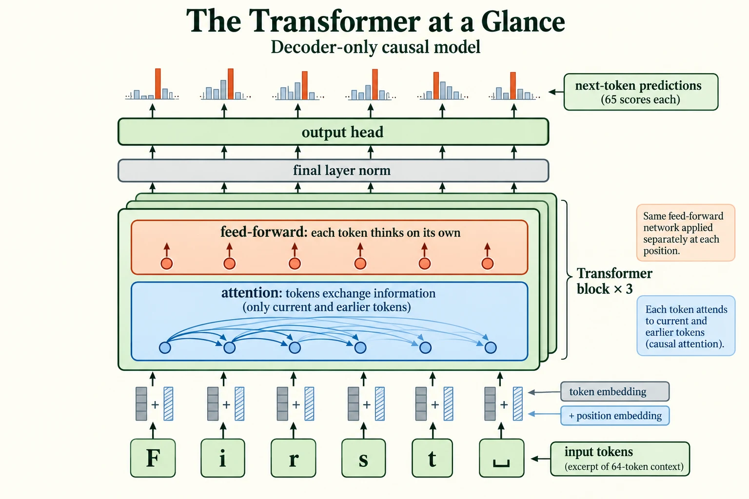
Figure 6.1.1. The lesson’s causal decoder-only Transformer adds token and position embeddings, applies three blocks, then normalises and predicts 65 next-character logits per position. The short row illustrates part of a 64-token context.
What does a Transformer block return for each input token?
A vector enriched by permitted context, with the same model width.
What Problem Were Transformers Designed to Address?
In Lesson 5.4 we found three problems with recurrent networks:
- A long chain: information, and the learning signal, has to pass through every step between two distant tokens, and fades along the way.
- A fixed-size bottleneck: everything read so far must be squeezed into one hidden state.
- Sequential computation: step 1,000 cannot start until step 999 has finished, so the parallel power of modern hardware is wasted.
The Transformer removes all three. Every token can attend directly to every other token, so the chain has length one. Every token keeps its own vector, so there is no single bottleneck. And because no token has to wait for the previous one, the whole sequence is processed at once. Let's see that last point concretely.
ids = torch.tensor([encode("First Citizen:\nBefore we proceed")]) # 32 characterswith torch.no_grad(): out = model(ids)print("predictions made in ONE forward pass:", out.shape[0] * out.shape[1], "(one per position)")print("an RNN would need", ids.shape[1], "sequential steps to read the same input")predictions made in ONE forward pass: 32 (one per position) an RNN would need 32 sequential steps to read the same input
For our 32-character input, a single forward pass of the Transformer produces 32 predictions at once: one at every position, each saying what character should come next at that point. An RNN reading the same input would need 32 steps, one after another.
This matters most during training. With one forward pass, we get a prediction, and therefore a training signal, at every position of every sequence in the batch. That is a key reason Transformers can be trained on enormous amounts of text. We return to this idea, called parallel training, in Lesson 6.6.
The price, as you saw at the end of Lesson 5.4, is that comparing every token with every other token costs work proportional to the square of the sequence length. We measure that cost in Lesson 6.3.
Which computation can causal Transformer training parallelise?
Predictions at known input positions in a training window.
The Transformer as a Complete Information-Processing System
Let's follow one input all the way through our model, and print the shape of the data after each stage. We use the first 32 characters of the play as input.
ids = torch.tensor([encode("First Citizen:\nBefore we proceed")]) # (1, T)print("input ids:", tuple(ids.shape))x = model.tok_emb(ids) + model.pos_emb(torch.arange(ids.shape[1]))print("after token + position embeddings:", tuple(x.shape))for i, block in enumerate(model.blocks.layers): x = block(x, src_mask=nn.Transformer.generate_square_subsequent_mask(ids.shape[1]), is_causal=True) print(f"after block {i + 1}:", tuple(x.shape))logits = model.head(model.ln_f(x))print("logits (one score per vocabulary entry, at every position):", tuple(logits.shape))input ids: (1, 32) after token + position embeddings: (1, 32, 64) after block 1: (1, 32, 64) after block 2: (1, 32, 64) after block 3: (1, 32, 64) logits (one score per vocabulary entry, at every position): (1, 32, 65)
Read the shapes from top to bottom:
- The input is
(1, 32): a batch of 1 sequence, 32 token IDs long. - After the embeddings it is
(1, 32, 64): each of the 32 tokens is now a vector of 64 numbers. This size, calledd_modelor the model dimension, is the "width" of the Transformer. - After each of the 3 blocks it is still
(1, 32, 64). Blocks never change the shape; they change the content of each token's vector, by mixing in information from other tokens. - After the output head it is
(1, 32, 65): at every one of the 32 positions, one score for each of the 65 characters in the vocabulary. These scores are called logits.
That constant shape inside the stack is one of the Transformer's most useful properties. Because each block takes (batch, tokens, d_model) and returns the same shape, you can stack as many blocks as you like, and the same block design works for any length of input up to the maximum context.
What does the untrained model predict? Let's turn the logits at the last position into probabilities with softmax and look at its best guesses for the character after "proceed".
with torch.no_grad(): probs = model(ids).softmax(-1)[0, -1] # distribution for the character after "proceed"top = probs.topk(5)print("untrained model's top-5 guesses for the next character:", [(repr(itos[i.item()]), round(p.item(), 3)) for p, i in zip(top.values, top.indices)])entropy = -(probs * probs.log()).sum().item()print(f"entropy of that distribution: {entropy:.3f} | maximum possible, ln({VOCAB}): {math.log(VOCAB):.3f}")untrained model's top-5 guesses for the next character: [("'i'", 0.065), ("'N'", 0.041), ("'R'", 0.035), ("' '", 0.03), ("'-'", 0.029)]
entropy of that distribution: 4.024 | maximum possible, ln(65): 4.174
The untrained model's favourite guess is 'i' with probability 0.065, followed by 'N', 'R', a space and '-'. These are random preferences, not knowledge. The entropy of the distribution, a measure of how spread out it is, is 4.024. The maximum possible, for a perfectly uniform guess among 65 characters, is ln(65) = 4.174. So the untrained model is close to "no idea at all", which is exactly where training will start from in Lesson 6.6.
Key terms
- Transformer: a network built from stacked blocks of attention and feed-forward layers that processes all tokens of a sequence in parallel.
- Model dimension (
d_model): the length of each token's vector inside the Transformer.- Transformer block: one round of attention plus feed-forward processing; input and output have the same shape.
- Logits: the raw scores the output head produces, one per vocabulary entry; softmax turns them into probabilities.
- Entropy: a measure of how uncertain a probability distribution is; highest when every outcome is equally likely.
-
If we fed our model a batch of 8 sequences, each 50 characters long, what would be the shape of the logits?
(8, 50, 65): 8 sequences, 50 positions each, and 65 scores (one per character) at every position.
What is the final axis of language-model logits?
One score per vocabulary entry.
The Roles of Tokens, Embeddings, Attention, and Feed-Forward Networks
Each stage of the pipeline has one job. Here they are in the order the data meets them:
- Tokens. The text is split into units and each unit gets an ID. The model only ever sees IDs. (Lesson 6.2.)
- Token embeddings. A lookup table turns each ID into a vector, exactly as in Lesson 5.3. This vector describes the token on its own, with no context.
- Positional information. Attention, as you will see in Lesson 6.3, has no built-in sense of order. So we add a second vector that encodes where each token sits. (Lessons 6.2 and 6.3.)
- Attention. Each token gathers information from other tokens, weighted by relevance. This is the only place where tokens exchange information. (Lesson 6.3.)
- Feed-forward network (FFN). A small two-layer MLP applied to each token's vector separately. It processes what attention gathered. (Lesson 6.4.)
- Output head. A linear layer that turns each final vector into one score per vocabulary entry. (Lesson 6.5.)
A useful slogan: attention moves information between tokens; the feed-forward network processes information within each token.
Where do the parameters live? Let's count them by component.
groups = {"token embedding": model.tok_emb, "position embedding": model.pos_emb}attn = sum(sum(p.numel() for p in l.self_attn.parameters()) for l in model.blocks.layers)ffn = sum(sum(p.numel() for n, p in l.named_parameters() if n.startswith("linear")) for l in model.blocks.layers)norms = sum(sum(p.numel() for n, p in l.named_parameters() if n.startswith("norm")) for l in model.blocks.layers) \ + sum(p.numel() for p in model.ln_f.parameters())rows = [("token embedding", model.tok_emb.weight.numel()), ("position embedding", model.pos_emb.weight.numel()), ("attention (3 blocks)", attn), ("feed-forward (3 blocks)", ffn), ("layer norms", norms), ("output head", sum(p.numel() for p in model.head.parameters()))]total = sum(n for _, n in rows)for name, n in rows: print(f"{name:<24} {n:>7,} {n / total:6.1%}")print(f"{'total':<24} {total:>7,}")token embedding 4,160 2.6% position embedding 4,096 2.5% attention (3 blocks) 49,920 30.7% feed-forward (3 blocks) 99,264 61.1% layer norms 896 0.6% output head 4,225 2.6% total 162,561
The feed-forward networks hold the most parameters: 99,264, or 61.1% of the model. Attention holds 49,920 (30.7%). The embeddings, output head and layer norms together hold well under a tenth. The roughly two-to-one ratio between feed-forward and attention follows from a standard design choice: each feed-forward network expands every vector to 4 × d_model numbers and back, which needs about twice as many weights as attention's four d_model × d_model projections. Large language models keep a similar balance, which is one reason researchers think of the feed-forward layers as the place where much of a model's "knowledge" is stored.
-
In one sentence each, what is the job of attention, and what is the job of the feed-forward network?
Attention moves information between tokens, letting each token gather what is relevant from the others. The feed-forward network processes the information within each token's vector, separately for every token.
Which component exchanges information between token positions?
Attention; the feed-forward network processes each resulting token vector separately.
Encoder, Decoder, and Encoder–Decoder Architectures
All Transformers share the blocks we have just seen. What distinguishes the three main families is which tokens each token is allowed to look at, and that is controlled by a mask: a grid that says, for every pair of positions, whether attention between them is allowed.
def mask_grid(kind, T=6, S=8): """Construct an illustrative allowed-attention grid for the selected Transformer family. Arguments: kind: The model or mask family selected in the surrounding example. T: Sequence length, or text-vector batch in contrastive_loss. S: Source-sequence length for the cross-attention grid. """ if kind == "encoder": return torch.ones(T, T) if kind == "decoder": return torch.tril(torch.ones(T, T)) return torch.ones(T, S) # cross-attention: target positions x source positionsfig, axes = plt.subplots(1, 3, figsize=(11, 3.6))for ax, (kind, title) in zip(axes, [("encoder", "Encoder self-attention\n(every token sees every token)"), ("decoder", "Decoder self-attention\n(causal: only earlier tokens)"), ("cross", "Cross-attention\n(output tokens see all input tokens)")]): g = mask_grid(kind) ax.pcolormesh(g, cmap="Blues", vmin=0, vmax=1.3, edgecolors="white", linewidth=1.5) ax.invert_yaxis(); ax.set_aspect("equal") ax.set_title(title, fontsize=9) ax.set_xlabel("input position being looked at" if kind == "cross" else "position being looked at") ax.set_ylabel("output position doing the looking" if kind == "cross" else "position doing the looking") ax.set_xticks(np.arange(g.shape[1]) + 0.5, range(g.shape[1])); ax.set_yticks(np.arange(g.shape[0]) + 0.5, range(g.shape[0]))plt.tight_layout(); plt.show()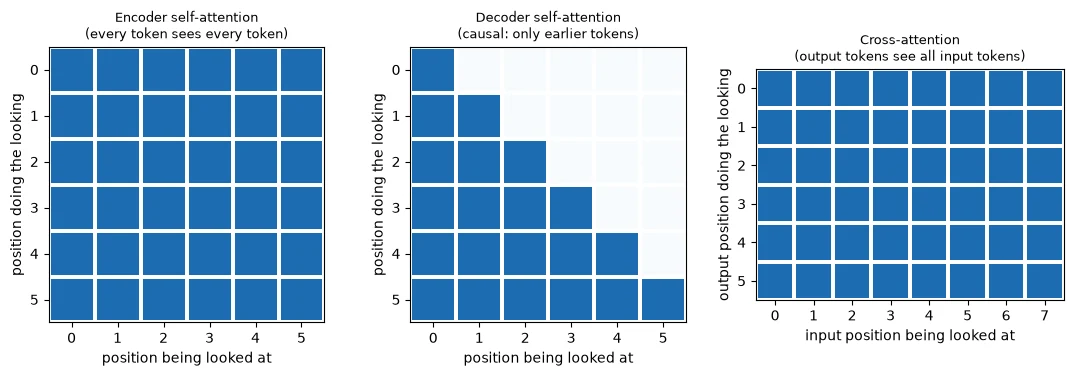
The three grids show the three patterns. Each row is a position doing the looking; each column is a position being looked at; blue means "allowed".
Encoder-only (bidirectional). Every token may look at every other token, before and after it (left grid). This gives the richest possible understanding of a complete input, so encoders are used to understand text: classify it, extract information from it, or produce embeddings for search. The best-known example is BERT. An ordinary bidirectional encoder is not trained for the left-to-right autoregressive generation loop we build here. It can predict masked tokens, and encoder architectures can be adapted for other generation procedures; "encoder" does not mean that text generation is fundamentally impossible.
Decoder-only (causal). Each token may look only at itself and the tokens before it (middle grid). This is called a causal mask, because the output at each position can only depend on what came earlier, just as a writer can only build on what has already been written. This is exactly what you need to generate text one token at a time. GPT-style language models, including the chat assistants you may have used, are decoder-only. So is the model we build in this module.
Encoder–decoder. An encoder reads the whole input bidirectionally; a decoder generates the output causally, and at every layer it also looks at the encoder's output through cross-attention (right grid: every output position may look at every input position). This suits tasks that turn one sequence into another, such as translation or summarisation. The original Transformer was of this kind; T5 is a well-known modern example.
We can verify the difference between bidirectional and causal attention directly. Below, two inputs differ only in their last character: "the king is dead" and "the king is deaf". We run both through our model with and without the causal mask, and check whether the output at the first position changes.
a = torch.tensor([encode("the king is dead")])b = torch.tensor([encode("the king is deaf")]) # only the LAST character differswith torch.no_grad(): for causal, name in [(False, "encoder-style (bidirectional)"), (True, "decoder-style (causal)")]: diff = (model(a, causal=causal)[0, 0] - model(b, causal=causal)[0, 0]).abs().max().item() print(f"{name:<31} change in the output at position 0: {diff:.6f}")encoder-style (bidirectional) change in the output at position 0: 0.095371 decoder-style (causal) change in the output at position 0: 0.000000
With bidirectional attention, changing the last character changes the output at position 0 (by up to 0.095371): the first token can "see" the end of the sentence. With the causal mask, the change is exactly 0.000000: the first token cannot see anything after it. The mask does exactly what it promises.
For completeness, here is PyTorch's full encoder–decoder nn.Transformer, with a source sequence of 10 tokens (say, an English sentence) and the first 7 tokens of a target sequence (its translation, generated so far):
torch.manual_seed(0)seq2seq = nn.Transformer(d_model=64, nhead=4, num_encoder_layers=2, num_decoder_layers=2, dim_feedforward=256, batch_first=True)src = torch.randn(1, 10, 64) # e.g. an English sentence of 10 tokens, already embeddedtgt = torch.randn(1, 7, 64) # the first 7 tokens of its French translationout = seq2seq(src, tgt, tgt_mask=nn.Transformer.generate_square_subsequent_mask(7))print("source:", tuple(src.shape), "| target so far:", tuple(tgt.shape), "| decoder output:", tuple(out.shape))source: (1, 10, 64) | target so far: (1, 7, 64) | decoder output: (1, 7, 64)
The decoder produces one vector per target position, (1, 7, 64), each informed by all 10 source tokens through cross-attention. To generate the 8th target token, a head would turn the last of these vectors into scores over the target vocabulary.
Key terms
- Mask: a grid that allows or blocks attention between each pair of positions.
- Bidirectional attention: every token can attend to every other token (encoders).
- Causal attention: each token can attend only to itself and earlier tokens (decoders).
- Cross-attention: attention from the decoder's tokens to the encoder's output.
- Encoder-only / decoder-only / encoder–decoder: the three Transformer families, used respectively for understanding, generating, and transforming one sequence into another.
-
Which family would you choose for each task: (a) deciding whether an email is spam; (b) a chatbot; (c) translating German into English?
(a) Encoder-only: you need to understand a complete email, not generate text. (b) Decoder-only: a chatbot generates its reply one token at a time. (c) Encoder–decoder: an encoder reads the whole German sentence and a decoder generates the English one, using cross-attention to consult the German. (Large decoder-only models can also translate, by treating the German text and its translation as one long sequence.)
What distinguishes ordinary encoder and decoder self-attention?
Bidirectional versus causally restricted access to input positions.
How Information Flows Through a Transformer
There is a powerful way to picture what happens inside the stack of blocks. Think of each token's vector as a stream that flows upward through the model. This is often called the residual stream. Each block does not replace the stream; it adds something to it: first whatever attention gathered from other tokens, then whatever the feed-forward network computed. (This "adding" is the residual connection, which you will meet properly in Lesson 6.4.)
So a token's vector starts as "this is the character d at position 8", and after each block it carries a little more about its surroundings. Let's watch this happen. We take two inputs with the same ending, "good lord" and "evil lord". Their final character, d, has the same ID and sits at the same position in both, so before any block their vectors must be identical. Do they stay identical?
s1 = torch.tensor([encode("good lord")])s2 = torch.tensor([encode("evil lord")])pos = 8 # the final 'd' sits at position 8 in bothprint(repr(decode(s1[0].tolist())[pos]), repr(decode(s2[0].tolist())[pos]))with torch.no_grad(): h1 = model.tok_emb(s1) + model.pos_emb(torch.arange(s1.shape[1])) h2 = model.tok_emb(s2) + model.pos_emb(torch.arange(s2.shape[1])) mask = nn.Transformer.generate_square_subsequent_mask(s1.shape[1]) print(f"before any block: cosine of the two 'd' vectors = {F.cosine_similarity(h1[0, pos], h2[0, pos], dim=0):.3f}") for i, block in enumerate(model.blocks.layers): h1 = block(h1, src_mask=mask, is_causal=True); h2 = block(h2, src_mask=mask, is_causal=True) print(f"after block {i + 1}: cosine of the two 'd' vectors = {F.cosine_similarity(h1[0, pos], h2[0, pos], dim=0):.3f}")'d' 'd' before any block: cosine of the two 'd' vectors = 1.000 after block 1: cosine of the two 'd' vectors = 0.997 after block 2: cosine of the two 'd' vectors = 0.989 after block 3: cosine of the two 'd' vectors = 0.978
Before any block, the cosine similarity of the two d vectors is 1.000: identical, as expected. After block 1 it is 0.997, after block 2 0.989, and after block 3 0.978. Because each block mixes in information from earlier tokens, the d in "good lord" and the d in "evil lord" gradually become different vectors. This is a contextual representation, the thing that static embeddings could not provide in Lesson 5.3.
The effect is small here because the model is untrained: its attention is essentially random, so it mixes in context weakly and without purpose. After training, the context will matter far more.
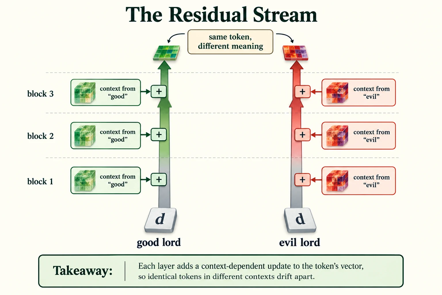
Figure 6.1.2. A schematic residual stream: the same character can acquire different context-dependent representations. The coloured updates are an analogy, not measured semantic coordinates or guaranteed attention behaviour.
-
Why must the two
dvectors be identical before the first block?Before the first block, a token's vector is just its token embedding plus its position embedding. Both
dtokens have the same ID and the same position (8), so they get exactly the same two vectors and the same sum. No information from other tokens has been mixed in yet.
What does each residual sub-layer add?
A computed update to the existing token-vector stream.
The Original Transformer vs. Modern Transformer Architectures
This section is included in class. It connects our teaching model to refinements used in research papers and model documentation.
The Transformer in "Attention Is All You Need" has been refined in several ways since it was published, mostly to make large models train more reliably:
- Where normalisation goes. The original placed layer normalisation after each attention and feed-forward step ("post-norm"). Most modern models place it before each step ("pre-norm"), which trains more stably in deep stacks. You will measure this difference yourself in Lesson 6.4.
- Activation function. The original feed-forward network used ReLU; modern models usually use smoother functions such as GELU or gated variants.
- Positional information. The original added fixed sine-and-cosine patterns. Many models instead learn position vectors, as ours does, and many large models use methods such as rotary position embeddings (RoPE) that encode relative positions inside attention itself.
- Families. The original was an encoder–decoder for translation. The most prominent models today are decoder-only.
These are refinements, not a different architecture. PyTorch builds both styles from the same layer class, with exactly the same number of parameters:
original = nn.TransformerEncoderLayer(64, 4, 256, dropout=0.0, activation="relu", batch_first=True, norm_first=False)modern = nn.TransformerEncoderLayer(64, 4, 256, dropout=0.0, activation="gelu", batch_first=True, norm_first=True)count = lambda m: sum(p.numel() for p in m.parameters())print("original-style layer (post-norm, ReLU):", count(original), "parameters")print("modern-style layer (pre-norm, GELU): ", count(modern), "parameters")original-style layer (post-norm, ReLU): 49984 parameters modern-style layer (pre-norm, GELU): 49984 parameters
Both layers have 49,984 parameters. The only differences are the order of operations (norm_first) and the activation function: the same components, arranged slightly differently.
What is pre-norm?
Normalising the input of a sub-layer before adding its output to the residual stream.
Beyond Text: Vision Transformers and Multimodal Models
Nothing in a Transformer block is specific to text. A block only needs a sequence of vectors. So if you can turn something into a sequence of vectors, you can process it with a Transformer.
The Vision Transformer (ViT) does exactly this for images. It cuts an image into a grid of small square patches, flattens each patch into a list of pixel values, and passes each through a linear layer to make a vector. Those patch vectors are then treated just like word embeddings. Here is the idea applied to a 28×28 Fashion-MNIST image, cut into 7×7 patches:
URL = "https://raw.githubusercontent.com/zalandoresearch/fashion-mnist/master/data/fashion/t10k-images-idx3-ubyte.gz"os.makedirs("data/fashion", exist_ok=True)FP = "data/fashion/t10k-images-idx3-ubyte.gz"if not os.path.exists(FP): urllib.request.urlretrieve(URL, FP)with gzip.open(FP) as fh: img = torch.tensor(np.frombuffer(fh.read(), np.uint8, offset=16)[:784].reshape(28, 28), dtype=torch.float32) / 255P = 7patches = img.unfold(0, P, P).unfold(1, P, P) # (4, 4, 7, 7): a 4x4 grid of 7x7 patchestokens = patches.reshape(-1, P * P) # (16, 49): 16 "tokens", 49 numbers eachprint("image:", tuple(img.shape), "| patches:", tuple(patches.shape), "| patch tokens:", tuple(tokens.shape))patch_embed = nn.Linear(P * P, D_MODEL)with torch.no_grad(): seq = patch_embed(tokens).unsqueeze(0) # (1, 16, 64): now looks exactly like a text sequence out = model.blocks.layers[0](seq) # the same kind of block, no maskprint("patch embeddings:", tuple(seq.shape), "-> after a Transformer block:", tuple(out.shape))fig, axes = plt.subplots(2, 1, figsize=(9, 5.4), gridspec_kw={"height_ratios": [3, 1]})axes[0].imshow(img, cmap="gray")for k in range(1, 4): axes[0].axhline(k * P - 0.5, color="orange"); axes[0].axvline(k * P - 0.5, color="orange")axes[0].set_title("image cut into 16 patches"); axes[0].axis("off")strip = torch.cat([torch.cat([patches[r, c], torch.ones(P, 1)], 1) for r in range(4) for c in range(4)], 1)axes[1].imshow(strip, cmap="gray"); axes[1].set_title("the same patches as a sequence of 16 tokens"); axes[1].axis("off")plt.tight_layout(); plt.show()image: (28, 28) | patches: (4, 4, 7, 7) | patch tokens: (16, 49) patch embeddings: (1, 16, 64) -> after a Transformer block: (1, 16, 64)
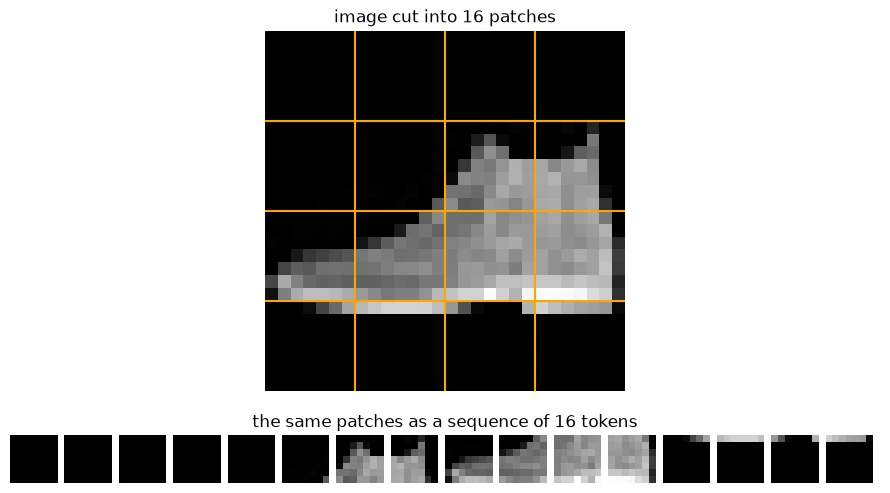
The 28×28 image becomes a 4×4 grid of patches, (4, 4, 7, 7), which we flatten into a sequence of 16 "tokens" of 49 numbers each, (16, 49). A linear layer turns each into a 64-number vector, giving (1, 16, 64): exactly the shape of a 16-token text sequence. We can then pass it through the same kind of Transformer block we used for Shakespeare, and get back (1, 16, 64). (In a real ViT, a position embedding is added too, so the model knows where each patch came from.)
Notice how this connects back to Module 5. A CNN builds in the assumption that nearby pixels belong together. A ViT does not: from its first layer, any patch can attend to any other patch. With enough training data, this flexibility pays off, which is why many modern vision models are Transformers.
The same trick powers multimodal models. Turn image patches, audio frames or video frames into vectors, put them in the same sequence as text tokens, and one Transformer can attend across all of them. That is how assistants that "see" an uploaded image work: the image becomes a set of vectors placed alongside the words of your question.
-
A 224×224 image is cut into 16×16 patches. How many patch tokens does the Vision Transformer receive?
224 / 16 = 14 patches along each side, so 14 × 14 = 196 patch tokens.
How does a Vision Transformer obtain patch tokens?
Flatten each patch and project it into the model's vector width.
Putting It All Together
A Transformer is a pipeline. Text is split into tokens and converted to IDs. Token embeddings and position embeddings turn each ID into a vector of size d_model. A stack of Transformer blocks then refines every token's vector: in each block, attention moves information between tokens and a feed-forward network processes each token on its own, and both add their results to the token's residual stream. Finally, an output head turns each vector into one score per vocabulary entry.
In our small model, a 32-character input flowed through as (1, 32) → (1, 32, 64) → three blocks that kept that shape → (1, 32, 65) logits: 32 next-character predictions from a single forward pass. Of its 162,561 parameters, 61.1% sit in the feed-forward networks and 30.7% in attention.
What separates the Transformer families is the mask. Encoders let every token see every token, which is ideal for understanding. Decoders use a causal mask, so each token sees only the past, which is needed for generation; we confirmed that a change at the end of the input left the first position's output exactly unchanged. Encoder–decoders combine the two with cross-attention. And because blocks only need a sequence of vectors, the same design works for image patches and mixed modalities.
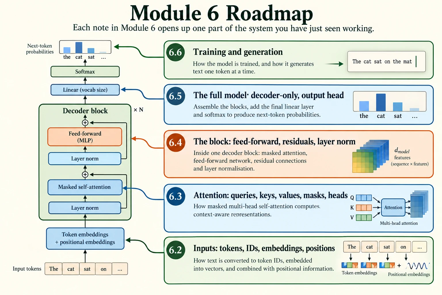
Figure 6.1.3. Follow the same system from inputs (6.2), through attention (6.3), the block (6.4), the full architecture (6.5), and training and generation (6.6). All Module 6 material is covered in class.
Summary
- A Transformer turns a sequence of tokens into a sequence of enriched vectors and then into predictions: tokens → embeddings (+ positions) → stacked blocks → output head.
- It was designed to remove the problems of recurrent networks: long chains, a fixed-size memory and sequential computation. It processes every position in parallel.
- Each block keeps the shape
(batch, tokens, d_model), so blocks can be stacked freely. - Attention moves information between tokens; the feed-forward network processes each token separately. In our model, the feed-forward networks hold 61.1% of the parameters.
- Encoder-only models see in both directions (understanding), decoder-only models use a causal mask (generation), and encoder–decoder models connect the two with cross-attention (sequence-to-sequence tasks).
- Each block adds to a token's residual stream, gradually turning identical tokens in different contexts into different, contextual vectors.
- Modern Transformers refine the original with pre-norm, GELU and new position methods. Vision Transformers apply the same blocks to sequences of image patches.
Glossary
| Term | Meaning |
|---|---|
| Transformer | A network of stacked attention and feed-forward blocks that processes all tokens in parallel. |
| Token / token ID | A unit of text, and its number in the vocabulary. |
| Token embedding | A learned vector for each token ID. |
| Position embedding | A vector added to each token's embedding to encode its position. |
d_model |
The length of each token's vector inside the model. |
| Transformer block | One layer of attention plus a feed-forward network, with the same input and output shape. |
| Attention | The mechanism by which tokens gather information from other tokens, weighted by relevance. |
| Feed-forward network (FFN) | A small MLP applied separately to each token's vector. |
| Output head | The final linear layer that turns vectors into vocabulary scores. |
| Logits | Raw output scores, before softmax. |
| Entropy | A measure of how spread out a probability distribution is. |
| Mask | A grid that allows or blocks attention between pairs of positions. |
| Causal mask | A mask that lets each position see only itself and earlier positions. |
| Encoder / decoder | A stack using bidirectional / causal self-attention. |
| Cross-attention | Attention from decoder tokens to encoder outputs. |
| Residual stream | A token's vector viewed as a stream that each block adds to. |
| Pre-norm / post-norm | Layer normalisation placed before / after each sub-layer. |
| Vision Transformer (ViT) | A Transformer that treats image patches as tokens. |
| Multimodal | Involving more than one type of data, such as images and text. |
Wrap-up
Quick check
What does a Transformer block return for each input token?
A vector enriched by permitted context, with the same model width.
What distinguishes ordinary encoder and decoder self-attention?
Bidirectional versus causally restricted access to input positions.
How does a Vision Transformer obtain patch tokens?
Flatten each patch and project it into the model's vector width.
Questions and discussion
Ask about this lesson, share what you found in a lab, or help someone else. Posts are public on the course's GitHub Discussions: anyone can read them, and you need a GitHub account to post.
Opening it loads giscus from giscus.app.