Building and Training an MLP You Can Defend
- Time
- ~117 min
- Sections
- 10
- Code cells
- 52
- Labs
- 5
- Figures
- 6
Before you start
You build a real MLP for the Bank Marketing data and defend every choice: how nn.Module registers parameters (and the silent bug when
it doesn't), how to compose blocks, how to trace shapes with hooks, why the loss takes logits, a training loop with correct bookkeeping,
a validation loop protected by eval() + no_grad(), an honest comparison with logistic regression, checkpoints you can resume,
and three modifications you write yourself: class weighting, an extra metric and early stopping.
- Goal
Build a multilayer perceptron (MLP) on real, imbalanced tabular data, train it with a loop you wrote yourself, and be able to defend every important choice in that loop — including the choice of whether the network was worth building at all.
An MLP (multilayer perceptron) is a feed-forward neural network made from fully connected (
Linear) layers and usually nonlinear activation functions such as ReLU. “Feed-forward” means information moves from the input toward the output; the network does not contain a recurrent memory of previous examples.This lesson is deliberately about mechanics and reasoning. You are not expected to memorise PyTorch APIs without understanding what they are doing. Whenever a technical term first appears, the note explains the idea first and then gives the term you will see in the code.
- Outcome
By the end of this lesson you will have a trained model, a checkpoint you could resume from, learning curves you can read, and an honest comparison against two baselines. You will also modify the training loop rather than only run it. That ability to change and defend the loop is Module 2’s end-of-module competency.
- You will be able to
- inspect a model with
parameters()andnamed_parameters(), and count its trainable parameters by hand; - explain parameter registration: how PyTorch keeps track of the weights, biases, and child layers that belong to a model;
- compose layers with
nn.Sequential, reusable sub-modules,ModuleList, and nested module trees; - trace shapes through a network with a dry run and forward hooks before real data touches it;
- choose between a one-logit and a two-logit output head and explain the corresponding label and loss conventions;
- explain what a logit is and why
BCEWithLogitsLossis preferable to manually applyingsigmoidand thenBCELossduring training; - write a training loop with correct gradient handling, loss accumulation, and
.item()discipline; - explain exactly what
loss.backward()calculates and why gradients are needed by the optimizer; - write a validation pass protected by
model.eval()andtorch.no_grad(), and explain why those two operations solve different problems; - read learning curves and identify mild overfitting without reaching for a fix before diagnosing the problem;
- evaluate an imbalanced classifier against a majority-class baseline and a logistic regression baseline;
- distinguish ranking quality from classification at a chosen threshold, and connect ranking to a limited call-centre capacity;
- save and resume a checkpoint containing model weights, optimizer state, epoch, and configuration;
- modify the loop yourself: class weighting, a new per-epoch metric, gradient inspection, and early stopping.
- inspect a model with
- Runtime
Section Approximate time Setup and data loading 10–60 s (60 only if re-downloading) Sections 1–4 — model construction and inspection under 10 s Section 7 — the 30-epoch training run ~20 s on CPU Section 9 — three modified runs ~30 s combined Everything else under 10 s Total execution is roughly two minutes on CPU. The models here are small on purpose: a 50→64→32→1 network has about 5,400 trainable parameters.
A parameter is a numerical value inside the model that training is allowed to change, usually a weight or bias. “5,400 parameters” therefore means the optimizer has roughly 5,400 trainable numbers available to adjust.
The point of Module 2 is not to train a large model. It is to understand the machinery well enough that, when a larger model fails, you know what the machinery is supposed to be doing.
Loading the data
If Lesson 2.2 ran in this working directory, bank_processed.npz is already there. If not — for example, in a fresh Colab session or after clearing the runtime — the fallback rebuilds it from the raw CSV using the same split, encoding, scaling, and random seed.
The important idea here is reproducibility. A fixed seed and a fixed preprocessing procedure let us recreate the same train/validation/test construction rather than silently changing the experiment each time the notebook is opened.
The three splits have different jobs:
- training set: used to calculate gradients and change model parameters;
- validation set: used while developing the model to compare choices and monitor generalisation;
- test set: held back for the final assessment. We do not use it to choose the model or training epoch in this lesson.
PROCESSED = DATA_DIR / "bank_processed.npz"BANK_CSV = DATA_DIR / "bank-full.csv"BANK_URL = "https://archive.ics.uci.edu/static/public/222/bank+marketing.zip"def rebuild_from_raw() -> dict: """Rebuild Lesson 2.2's processed dataset from the raw CSV (used only if the .npz is missing). Downloads UCI Bank Marketing if needed, drops the leaky ``duration`` column, makes the same stratified 70/15/15 split with the same seed, one-hot encodes the categoricals and standardises the numerics with statistics from the training split only. Returns: A dict with ``X_train``, ``y_train``, ``X_val``, ``y_val``, ``X_test``, ``y_test`` (float32 feature matrices and int64 label vectors) and ``feature_names``. """ if not BANK_CSV.exists(): print("Downloading UCI Bank Marketing ...") outer = DATA_DIR / "bank+marketing.zip" urllib.request.urlretrieve(BANK_URL, outer) with zipfile.ZipFile(outer) as z: z.extract("bank.zip", DATA_DIR) with zipfile.ZipFile(DATA_DIR / "bank.zip") as z: z.extract("bank-full.csv", DATA_DIR) outer.unlink() (DATA_DIR / "bank.zip").unlink() df = pd.read_csv(BANK_CSV, sep=";").drop(columns=["duration"]) # target leak y_all = (df.pop("y") == "yes").astype(np.int64).values numeric = [c for c in df.columns if df[c].dtype.kind in "iuf"] categorical = [c for c in df.columns if c not in numeric] X_tr, X_tmp, y_tr, y_tmp = train_test_split( df, y_all, test_size=0.30, stratify=y_all, random_state=SEED) X_va, X_te, y_va, y_te = train_test_split( X_tmp, y_tmp, test_size=0.50, stratify=y_tmp, random_state=SEED) train_ohe = pd.get_dummies(X_tr, columns=categorical) names = list(train_ohe.columns) scaler = StandardScaler().fit(train_ohe[numeric]) def finish(frame): """Encode one split exactly like the training split. Args: frame: A split of the original DataFrame (features only). Returns: A float32 array with the training feature columns: one-hot categoricals aligned to the training columns and numerics transformed by the training scaler. """ out = pd.get_dummies(frame, columns=categorical).reindex( columns=names, fill_value=0).astype(np.float32) out[numeric] = scaler.transform(out[numeric]).astype(np.float32) return out.values.astype(np.float32) return dict( X_train=finish(X_tr), y_train=y_tr, X_val=finish(X_va), y_val=y_va, X_test=finish(X_te), y_test=y_te, feature_names=np.array(names, dtype=object), )if PROCESSED.exists(): print(f"Loading {PROCESSED} (produced by Note 2.2)") blob = dict(np.load(PROCESSED, allow_pickle=True))else: print(f"{PROCESSED} not found — rebuilding from the raw CSV") blob = rebuild_from_raw() np.savez_compressed(PROCESSED, **blob)X_train, y_train = blob["X_train"], blob["y_train"]X_val, y_val = blob["X_val"], blob["y_val"]X_test, y_test = blob["X_test"], blob["y_test"]feature_names = list(blob["feature_names"])N_FEATURES = X_train.shape[1]for name, X_, y_ in [("train", X_train, y_train), ("val", X_val, y_val), ("test", X_test, y_test)]: print(f" {name:<6} {X_.shape[0]:>6,} x {X_.shape[1]} positive rate {y_.mean():.4f}")Loading data/bank_processed.npz (produced by Note 2.2) train 31,647 x 50 positive rate 0.1170 val 6,782 x 50 positive rate 0.1171 test 6,782 x 50 positive rate 0.1169
X_valarray([[ 0.85833985, -0.59722406, 0.38330433, ..., 0. ,
0. , 0. ],
[ 0.199308 , -0.46465886, 0.26326996, ..., 1. ,
0. , 0. ],
[-0.36557648, 0.28382978, 0.50333863, ..., 0. ,
0. , 0. ],
...,
[ 0.76419246, -0.3438193 , -1.4172109 , ..., 0. ,
0. , 1. ],
[-1.2129033 , -0.59722406, -1.0571078 , ..., 0. ,
0. , 1. ],
[ 1.4232243 , 1.4348999 , 0.50333863, ..., 0. ,
0. , 1. ]], shape=(6782, 50), dtype=float32)
BATCH_SIZE = 256def to_loader(X, y, batch_size, shuffle): """Wrap feature and label arrays in a DataLoader that yields ``(x, y)`` batches. Labels are converted to float and reshaped to ``(N, 1)`` so they match a one-logit output and ``BCEWithLogitsLoss``. Args: X: Float32 feature matrix of shape ``(N, F)``. y: Integer label vector of shape ``(N,)``. batch_size: Examples per batch. shuffle: ``True`` for training, ``False`` for validation and test. Returns: A ``DataLoader`` over a ``TensorDataset``. """ ds = TensorDataset( torch.from_numpy(X), torch.from_numpy(y).float().unsqueeze(1), # (N, 1) to match a 1-logit head ) return DataLoader(ds, batch_size=batch_size, shuffle=shuffle)seed_everything(SEED)train_loader = to_loader(X_train, y_train, BATCH_SIZE, shuffle=True)val_loader = to_loader(X_val, y_val, 1024, shuffle=False)test_loader = to_loader(X_test, y_test, 1024, shuffle=False)xb, yb = next(iter(train_loader))assert xb.shape == (BATCH_SIZE, N_FEATURES) and xb.dtype == torch.float32assert yb.shape == (BATCH_SIZE, 1) and yb.dtype == torch.float32print(f"train {len(train_loader)} batches | val {len(val_loader)} | test {len(test_loader)}")print(f"one batch: x {tuple(xb.shape)} {xb.dtype}, y {tuple(yb.shape)} {yb.dtype} — contract holds")train 124 batches | val 7 | test 7 one batch: x (256, 50) torch.float32, y (256, 1) torch.float32 — contract holds
Setup — imports, versions and device detection used by the notebook (2 cells)
# Pinned for reproducibility. Uncomment to install in a fresh environment (Colab / Kaggle).# !pip install -q torch==2.14.0 numpy==2.4.4 pandas==3.0.2 scikit-learn==1.8.0 matplotlib==3.10.8import osimport sysimport timeimport copyimport zipfileimport urllib.requestfrom pathlib import Pathimport numpy as npimport pandas as pdimport torchimport torch.nn as nnimport matplotlib.pyplot as pltfrom torch.utils.data import TensorDataset, DataLoaderimport sklearnfrom sklearn.model_selection import train_test_splitfrom sklearn.preprocessing import StandardScalerfrom sklearn.linear_model import LogisticRegressionfrom sklearn.metrics import ( roc_auc_score, average_precision_score, precision_recall_curve, roc_curve, confusion_matrix, f1_score,)print(f"python : {sys.version.split()[0]}")print(f"torch : {torch.__version__}")print(f"numpy : {np.__version__}")print(f"pandas : {pd.__version__}")print(f"scikit-learn : {sklearn.__version__}")python : 3.13.9 torch : 2.14.0 numpy : 2.3.5 pandas : 2.3.3 scikit-learn : 1.7.2
def get_device() -> torch.device: """Return the best available device: CUDA, then Apple MPS, then CPU. Returns: A ``torch.device`` for the fastest backend on this machine. """ if torch.cuda.is_available(): return torch.device("cuda") if torch.backends.mps.is_available() and torch.backends.mps.is_built(): return torch.device("mps") return torch.device("cpu")def seed_everything(seed: int = 42) -> None: """Seed every random-number generator that affects training. Sets Python's hash seed, NumPy and PyTorch (plus all CUDA devices when present), so data shuffling, weight initialisation and dropout repeat exactly for the same seed. Args: seed: The seed value to use everywhere. """ os.environ["PYTHONHASHSEED"] = str(seed) np.random.seed(seed) torch.manual_seed(seed) if torch.cuda.is_available(): torch.cuda.manual_seed_all(seed)SEED = 42DEVICE = get_device()seed_everything(SEED)DATA_DIR = Path("data")DATA_DIR.mkdir(exist_ok=True)CKPT_DIR = Path("checkpoints")CKPT_DIR.mkdir(exist_ok=True)print(f"Device: {DEVICE}")if DEVICE.type == "cuda": print(f" {torch.cuda.get_device_name(0)}")print(f"Seed : {SEED}")Device: mps Seed : 42
nn.Module past the introduction
You have already subclassed nn.Module, defined forward, and seen that the code works. The important question now is: what does nn.Module actually keep track of for us?
Start with the concrete idea. A neural network contains numerical values that training is allowed to change. Those values are the model’s parameters — for example, the weights and bias of a Linear layer.
PyTorch needs to know which objects inside your Python object are part of the neural network. When you assign a layer such as nn.Linear(...) to an attribute of an nn.Module inside __init__, PyTorch records that layer as a child module. The parameters inside that layer are then part of the model’s registered parameters.
This tracking is called parameter/module registration. It is not cosmetic bookkeeping. Later, several PyTorch operations rely on this record:
model.parameters()finds the trainable tensors that an optimizer should update;model.to(device)moves registered parameters and buffers to CPU, CUDA, or another device;state_dict()collects the registered model state so it can be saved;model.train()andmodel.eval()propagate the appropriate mode to child modules.
So when this lesson says that a layer is “registered”, read that as: PyTorch knows that this object belongs to the model and can include it in these model-management operations.
class TinyNet(nn.Module): """A minimal two-layer network used to show what ``nn.Module`` registers. Its two ``nn.Linear`` layers are registered as child modules (their weights appear in ``named_parameters()``); the plain float attribute ``dropout_rate`` is not. """ def __init__(self, in_features: int, hidden: int = 8): """Create and register the layers. Args: in_features: Number of input features. hidden: Width of the hidden layer. """ super().__init__() # ALWAYS first: sets up the registry self.fc1 = nn.Linear(in_features, hidden) self.fc2 = nn.Linear(hidden, 1) self.activation = nn.ReLU() self.dropout_rate = 0.0 # a plain float — NOT registered def forward(self, x): """Linear → ReLU → Linear. Args: x: Input of shape ``(N, in_features)``. Returns: Logits of shape ``(N, 1)``. """ return self.fc2(self.activation(self.fc1(x)))tiny = TinyNet(in_features=6, hidden=8)print(tiny)print()print("Registered parameters:")for name, p in tiny.named_parameters(): print(f" {name:<12} {str(tuple(p.shape)):<12} requires_grad={p.requires_grad}")print(f"\nself.dropout_rate = {tiny.dropout_rate} is a plain attribute.")print("It does not appear above, because it is not a Parameter or a Module.")TinyNet( (fc1): Linear(in_features=6, out_features=8, bias=True) (fc2): Linear(in_features=8, out_features=1, bias=True) (activation): ReLU() ) Registered parameters: fc1.weight (8, 6) requires_grad=True fc1.bias (8,) requires_grad=True fc2.weight (1, 8) requires_grad=True fc2.bias (1,) requires_grad=True self.dropout_rate = 0.0 is a plain attribute. It does not appear above, because it is not a Parameter or a Module.
The registry is what makes the optimizer possible
An optimizer is the object that changes model parameters after gradients have been calculated. Adam is one example.
When you write:
torch.optim.Adam(model.parameters(), ...)model.parameters() gives Adam the tensors it is allowed to update. This is why registration matters: if a layer’s parameters are not registered, the optimizer never receives them.
The dangerous part is that this usually does not produce an error. The model can still run a forward pass, calculate a loss, and run backward(). It simply leaves some weights unchanged. That is a silent training bug: the program runs, but the model is only partly learning.
class BrokenNet(nn.Module): """A deliberately buggy network: two hidden layers kept in a plain Python list. The list's layers run in ``forward`` but are *not registered*, so they are missing from ``model.parameters()``, never updated by the optimizer, not moved by ``.to()`` and not saved in ``state_dict()``. Only 65 of its 209 weights can learn. """ def __init__(self, in_features): """Create the layers, two of them in an unregistered Python list (the bug). Args: in_features: Number of input features. """ super().__init__() self.fc1 = nn.Linear(in_features, 8) self.hidden_layers = [nn.Linear(8, 8), nn.Linear(8, 8)] # a plain list! self.out = nn.Linear(8, 1) def forward(self, x): """Input layer, the two hidden layers from the list, then the output layer. Args: x: Input of shape ``(N, in_features)``. Returns: Logits of shape ``(N, 1)``. """ x = torch.relu(self.fc1(x)) for layer in self.hidden_layers: x = torch.relu(layer(x)) return self.out(x)class FixedNet(nn.Module): """The corrected ``BrokenNet``: the hidden layers live in an ``nn.ModuleList``. ``nn.ModuleList`` registers every module it holds, so all 209 parameters are visible to the optimizer, the device, and the saved state. """ def __init__(self, in_features): """Create the layers, holding the hidden ones in an ``nn.ModuleList``. Args: in_features: Number of input features. """ super().__init__() self.fc1 = nn.Linear(in_features, 8) self.hidden_layers = nn.ModuleList([nn.Linear(8, 8), nn.Linear(8, 8)]) self.out = nn.Linear(8, 1) def forward(self, x): """Input layer, each registered hidden layer with ReLU, then the output layer. Args: x: Input of shape ``(N, in_features)``. Returns: Logits of shape ``(N, 1)``. """ x = torch.relu(self.fc1(x)) for layer in self.hidden_layers: x = torch.relu(layer(x)) return self.out(x)def count_params(model): """Count the trainable numbers the optimizer can see in a model. Args: model: Any ``nn.Module``. Returns: The total number of elements across ``model.parameters()``: only registered parameters are counted. """ return sum(p.numel() for p in model.parameters())broken, fixed = BrokenNet(6), FixedNet(6)print(f"BrokenNet: {count_params(broken):>4} parameters visible to an optimizer")print(f"FixedNet : {count_params(fixed):>4} parameters visible to an optimizer")print(f"\nBoth run forward identically. Both produce a loss. Both call backward().")print(f"BrokenNet silently never updates {count_params(fixed) - count_params(broken)} of its weights.")x_demo = torch.randn(4, 6)print(f"\nforward works on both: broken {tuple(broken(x_demo).shape)}, " f"fixed {tuple(fixed(x_demo).shape)}")BrokenNet: 65 parameters visible to an optimizer FixedNet : 209 parameters visible to an optimizer Both run forward identically. Both produce a loss. Both call backward(). BrokenNet silently never updates 144 of its weights. forward works on both: broken (4, 1), fixed (4, 1)
That is the same category of bug as Lesson 2.1’s silent broadcast: the program runs, produces plausible numbers, and does not necessarily tell you that something is wrong. The defence is the same — check the structure instead of assuming it:
assert count_params(model) == expected, "parameter count mismatch"If you need a collection of layers, use a PyTorch container that knows it is holding modules:
nn.ModuleListis a list-like container for child modules;nn.ModuleDictis a dictionary-like container for named child modules.
A plain Python list or dictionary does not automatically register the modules it contains.
Why you call the module, not forward
model(x) vs model.forward(x)
model(x)Goes through nn.Module.__call__: runs registered hooks before and after forward and other bookkeeping. Always use this.
model.forward(x)Same numbers today, but skips the hooks. Tools that rely on them (shape tracing, profilers, some libraries) silently stop working.
There is another layer of machinery around forward. When you write:
model(x)Python invokes the module’s __call__ machinery, which in turn handles the forward pass and PyTorch features such as hooks. Calling model.forward(x) directly jumps past that machinery.
So the normal rule is simple: call the model as model(x), not model.forward(x). You define forward; PyTorch’s module interface decides how that forward computation is wrapped.
x_demo = torch.randn(4, 6)direct = tiny(x_demo) # correctbypass = tiny.forward(x_demo) # runs, gives the same numbers, skips machineryprint(f"tiny(x) -> {tuple(direct.shape)}")print(f"tiny.forward(x) -> {tuple(bypass.shape)}")print(f"identical values: {torch.equal(direct, bypass)}")print()print("Calling the module invokes __call__, which runs registered hooks around forward().")print("Calling .forward() directly skips them. Section 3 uses hooks, so this matters.")tiny(x) -> (4, 1) tiny.forward(x) -> (4, 1) identical values: True Calling the module invokes __call__, which runs registered hooks around forward(). Calling .forward() directly skips them. Section 3 uses hooks, so this matters.
-
BrokenNetandFixedNetdiffer by 144 parameters. If you trainedBrokenNet, would the loss go down at all? Predict, then reason about which layers are in the registry.Yes, the loss still goes down, just less. The registry holds
fc1(56 parameters) andout(9 parameters), so the optimizer adapts the first and last layers around two hidden layers frozen at their random initial weights. That's a bit like learning on top of random features: it can fit something, but far worse than a network whose middle layers learn too. The danger is exactly that it looks like training works. -
super().__init__()must come first. What specifically fails if you assignself.fc1before calling it?nn.Module.__init__creates the internal registries (_parameters,_modules,_buffers).nn.Module.__setattr__interceptsself.fc1 = …and tries to put the layer in_modules, which doesn't exist yet, so PyTorch raisesAttributeError: cannot assign module before Module.__init__() call.
Layers stored in a plain Python list, self.layers = [nn.Linear(...), ...]. What happens when you train?
A plain list does not register modules, so model.parameters() misses them. The forward pass and backward still run. Use nn.ModuleList.
Registration lets PyTorch do all of these except…
Registration is bookkeeping for parameters, devices, checkpoints and modes. The learning rate is still your choice.
Why is the plain-list bug described as 'silent', and how would you catch it?
- The model still runs forward, computes a loss and calls backward without errors; the unregistered weights simply never change, so it only partly learns.
- Catch it by checking structure: count
model.parameters()against the expected total, or printnamed_parameters().
Composing blocks
A network is easier to reason about when you can describe it as a sequence of reusable pieces rather than as one long expression.
There are three common ways to assemble a network, and they trade brevity against control:
nn.Sequential— useful when the data simply flows through a fixed sequence of layers;- a reusable sub-module — useful when a pattern such as
Linear → ReLUappears more than once; - a custom
nn.Modulewith named child modules — useful when the forward pass contains branching, skip/residual connections, multiple inputs, or other logic that a straight sequence cannot express.
The important idea is composition: a large model can be built from smaller modules, and those modules can themselves contain modules.
# --- Style A: nn.Sequential. Concise. No control flow in forward. ---seq_model = nn.Sequential( nn.Linear(N_FEATURES, 64), nn.ReLU(), nn.Linear(64, 32), nn.ReLU(), nn.Linear(32, 1),)seq_modelSequential( (0): Linear(in_features=50, out_features=64, bias=True) (1): ReLU() (2): Linear(in_features=64, out_features=32, bias=True) (3): ReLU() (4): Linear(in_features=32, out_features=1, bias=True) )
# --- Style B: an explicit subclass. Verbose. Full control. ---class ExplicitMLP(nn.Module): """The 50-64-32-1 MLP written as an explicit subclass (style B). Same architecture and parameter count as the ``nn.Sequential`` version, but the ``forward`` method is ordinary Python, so it could contain branches or skips. """ def __init__(self, in_features, h1=64, h2=32): """Create the two hidden layers, the output layer and the activation. Args: in_features: Number of input features. h1: Width of the first hidden layer. h2: Width of the second hidden layer. """ super().__init__() self.fc1 = nn.Linear(in_features, h1) self.fc2 = nn.Linear(h1, h2) self.out = nn.Linear(h2, 1) self.act = nn.ReLU() def forward(self, x): """Two Linear+ReLU layers, then the output layer. Args: x: Input of shape ``(N, in_features)``. Returns: Logits of shape ``(N, 1)``. """ x = self.act(self.fc1(x)) x = self.act(self.fc2(x)) return self.out(x)explicit = ExplicitMLP(N_FEATURES)print(f"Sequential : {count_params(seq_model):,} parameters")print(f"Explicit : {count_params(explicit):,} parameters")print("Same architecture, same count. The difference is what you can express in forward().")Sequential : 5,377 parameters Explicit : 5,377 parameters Same architecture, same count. The difference is what you can express in forward().
A reusable block, and why blocks matter
Real neural-network architectures often repeat the same small pattern. For this model the repeated pattern is essentially:
Linear → ReLU
Instead of writing that pattern repeatedly, we can package it into a small module called a block. A block is simply a reusable piece of a larger network.
The technical idea is composition: we construct a larger model by putting smaller modules together. This makes the model easier to read, inspect, change, and reuse. The same design idea appears in much larger architectures, including the repeated blocks used in Transformers.
class DenseBlock(nn.Module): """A reusable ``Linear → ReLU`` building block. Packaging the repeated motif once lets a larger model be described as a stack of blocks, which is the same idea that Transformers use at a larger scale. """ def __init__(self, in_features: int, out_features: int): """Create the linear layer and its activation. Args: in_features: Width of the block's input. out_features: Width of the block's output. """ super().__init__() self.linear = nn.Linear(in_features, out_features) self.act = nn.ReLU() def forward(self, x): """Apply the linear layer, then ReLU. Args: x: Input of shape ``(N, in_features)``. Returns: Activations of shape ``(N, out_features)``. """ return self.act(self.linear(x))class BankMLP(nn.Module): """The multilayer perceptron trained on Bank Marketing in this lesson. A stack of ``DenseBlock`` layers whose widths come from ``hidden_sizes``, followed by a linear head that outputs raw logits. Making the widths a constructor argument turns depth and width into configuration choices that can be stored in a checkpoint. Attributes: blocks: ``nn.ModuleList`` of ``DenseBlock`` layers. head: Final ``nn.Linear`` producing one logit per example (by default). """ def __init__(self, in_features: int, hidden_sizes=(64, 32), out_features: int = 1): """Build the blocks and the output head. Args: in_features: Number of input features (50 after encoding). hidden_sizes: Width of each hidden layer, in order, e.g. ``(64, 32)``. out_features: Number of outputs; 1 for a single binary logit. """ super().__init__() sizes = [in_features, *hidden_sizes] self.blocks = nn.ModuleList( DenseBlock(sizes[i], sizes[i + 1]) for i in range(len(hidden_sizes)) ) self.head = nn.Linear(sizes[-1], out_features) def forward(self, x): """Run the input through every block, then the head. Args: x: Input of shape ``(N, in_features)``. Returns: Raw logits of shape ``(N, out_features)``, with no sigmoid applied. """ for block in self.blocks: x = block(x) return self.head(x) # raw logits — no sigmoid, see Section 4N_FEATURES50
seed_everything(SEED)model = BankMLP(N_FEATURES, hidden_sizes=(64, 32))print(model)BankMLP(
(blocks): ModuleList(
(0): DenseBlock(
(linear): Linear(in_features=50, out_features=64, bias=True)
(act): ReLU()
)
(1): DenseBlock(
(linear): Linear(in_features=64, out_features=32, bias=True)
(act): ReLU()
)
)
(head): Linear(in_features=32, out_features=1, bias=True)
)
print("The module tree, and where the parameters live:\n")total = 0for name, p in model.named_parameters(): total += p.numel() print(f" {name:<24} {str(tuple(p.shape)):<12} {p.numel():>6,}")print(f" {'TOTAL':<24} {'':<12} {total:>6,}")by_hand = (N_FEATURES * 64 + 64) + (64 * 32 + 32) + (32 * 1 + 1)print(f"\nBy hand: ({N_FEATURES}x64 + 64) + (64x32 + 32) + (32x1 + 1) = {by_hand:,}")print(f"Matches: {by_hand == total}")print(f"\nMemory for the weights alone, float32: {total * 4 / 1024:.1f} KB")print("Adam also stores two running averages per parameter, so training")print(f"state is roughly 3x that: {total * 4 * 3 / 1024:.1f} KB. Day 4 budgets this properly.")The module tree, and where the parameters live: blocks.0.linear.weight (64, 50) 3,200 blocks.0.linear.bias (64,) 64 blocks.1.linear.weight (32, 64) 2,048 blocks.1.linear.bias (32,) 32 head.weight (1, 32) 32 head.bias (1,) 1 TOTAL 5,377 By hand: (50x64 + 64) + (64x32 + 32) + (32x1 + 1) = 5,377 Matches: True Memory for the weights alone, float32: 21.0 KB Adam also stores two running averages per parameter, so training state is roughly 3x that: 63.0 KB. Day 4 budgets this properly.
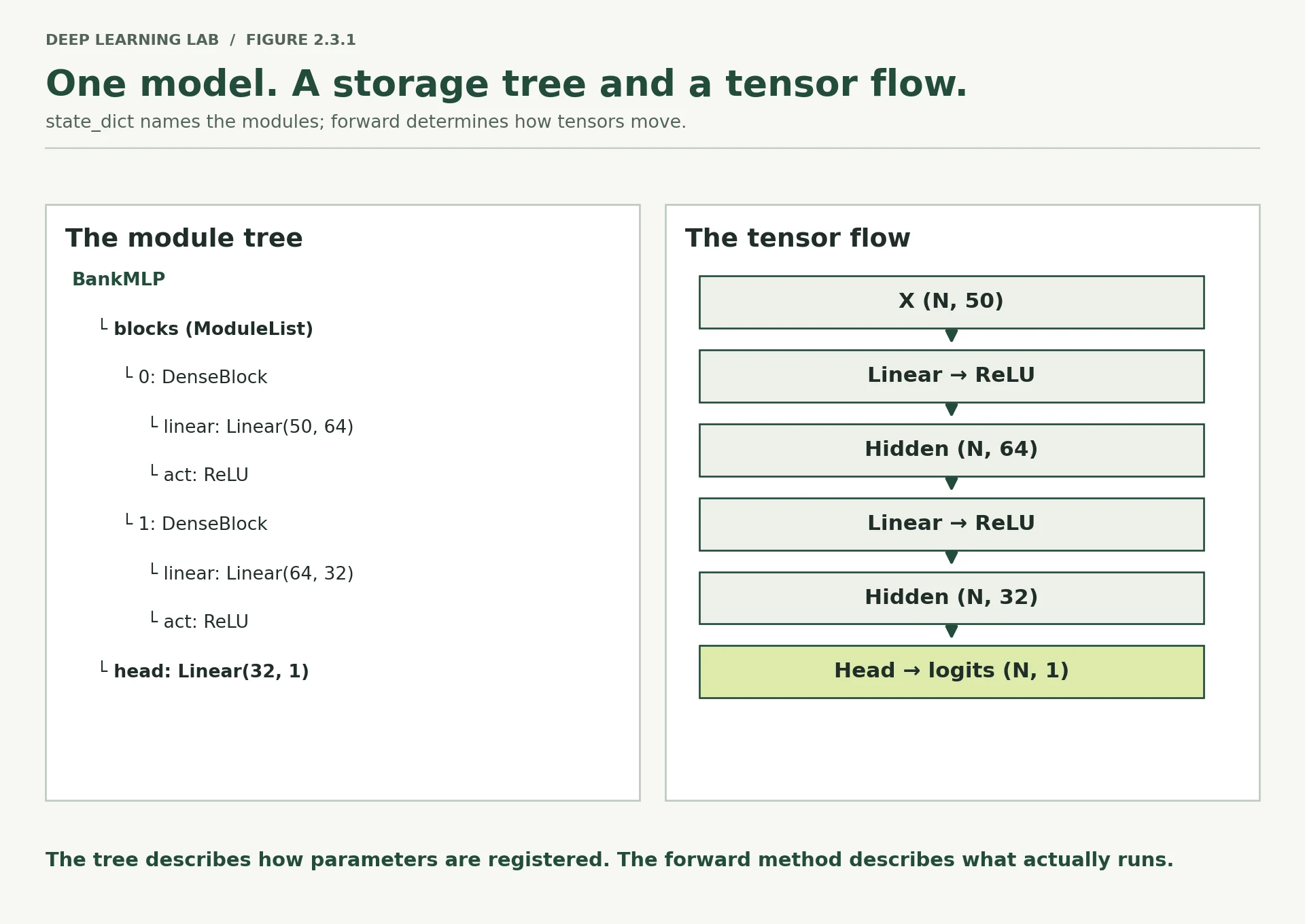
The dotted parameter names are not arbitrary labels. They describe the path through the module tree.
A module tree is simply the nested structure of the model. For example:
BankMLP
├── blocks
│   ├── 0
│   │   ├── linear
│   │   └── act
│   └── 1
│       ├── linear
│       └── act
└── head
So blocks.0.linear.weight means:
BankMLP→blocks→ block0→linearlayer → itsweighttensor.
Those paths become keys in state_dict(), which is PyTorch’s dictionary-like representation of the model state. This is why renaming a submodule can affect whether an old checkpoint loads cleanly: the saved keys may no longer match the new module-tree paths.
This is also why Section 8 saves the architecture configuration alongside the weights. The weights are meaningful only when we reconstruct the architecture they belong to.
-
BankMLP(N_FEATURES, hidden_sizes=(64, 32))has about 5,400 parameters. What doeshidden_sizes=(256, 128, 64)give you? Compute it before running it. Remember that eachLinearlayer has a weight matrix and, when enabled, a bias vector.Each layer is
in × out + out: \(50\times256+256 = 13{,}056\); \(256\times128+128 = 32{,}896\); \(128\times64+64 = 8{,}256\); head \(64\times1+1 = 65\) → 54,273 parameters, about 10× the(64, 32)model. Most of it sits in the 256→128 layer. Check it in the calculator above. -
nn.Sequentialcannot express a residual connection such asx + f(x)using only a simple chain. Why does that require access to the originalx, and what does that tell you about when to reach for a customnn.Module?A residual block computes
out = x + f(x): the input must still be available afterfhas run, so the forward pass has two paths (skip and transform) that meet again.nn.Sequentialonly passes each layer's output to the next, forgetting everything earlier. Whenever the data flow isn't a single straight chain (skips, branches, multiple inputs, conditional logic), write a customnn.Modulewith an explicitforward.
What does the parameter name blocks.0.linear.weight describe?
These paths are the keys in state_dict(), which is why renaming a sub-module can stop an old checkpoint loading.
When do you need a custom nn.Module rather than nn.Sequential?
Sequential is a straight chain. A residual connection needs the original \(x\) later in forward, which a chain cannot keep.
Tracing shapes through a model
Lesson 2.1’s shape clinic dealt with one layer at a time. In a real model, a shape mistake may originate several layers before the line that finally fails. The error message usually identifies the operation that could not proceed, not necessarily the earlier configuration choice that caused the mismatch.
The first tool is deliberately simple: dry-run a fake batch before you touch real data.
A dry run means sending artificial data through the model only to test the wiring. We do not care about the predictions. We care that the input shape is accepted and that the output shape is what the next stage expects.
def dry_run(model: nn.Module, in_features: int, batch_size: int = 2) -> torch.Tensor: """Push one fake batch through a model to check its wiring, not its predictions. Runs in evaluation mode without gradients and prints the input and output shapes. A wrong input width fails immediately with a readable shape error. Args: model: The model to test. in_features: Number of features in the fake input. batch_size: Rows in the fake batch. Returns: The model's output for the fake batch. Raises: RuntimeError: If any layer receives a shape it can't handle. """ model.eval() fake = torch.randn(batch_size, in_features) with torch.no_grad(): out = model(fake) print(f"dry run: in {tuple(fake.shape)} -> out {tuple(out.shape)}") return out_ = dry_run(model, N_FEATURES)# The same dry run against a WRONG feature count fails instantly and informatively.try: dry_run(model, N_FEATURES + 7)except RuntimeError as e: print(f"\nWrong input width caught immediately: {str(e)[:100]}")dry run: in (2, 50) -> out (2, 1) Wrong input width caught immediately: mat1 and mat2 shapes cannot be multiplied (2x57 and 50x64)
Forward hooks: seeing every intermediate shape
A hook is a function that PyTorch can call automatically when a particular event happens inside a module. A forward hook runs when a module has performed its forward computation, so it lets us inspect what went into a layer and what came out without rewriting the model.
Think of a forward hook as temporarily attaching a measuring instrument to a layer.
Register one on each leaf submodule and run one fake batch. You then get a trace of the tensor as it moves through the network.
This also explains why the earlier distinction between model(x) and model.forward(x) matters. Hooks are part of the module’s __call__ machinery. Calling forward directly bypasses that machinery, so a forward hook would not fire in the normal way.
def trace_shapes(model: nn.Module, in_features: int, batch_size: int = 4): """Print every leaf layer's input and output shape for one fake batch. Attaches a forward hook to each leaf module (a module without children), runs one batch, removes the hooks and prints a table in execution order. Args: model: The model to trace. in_features: Number of features in the fake input. batch_size: Rows in the fake batch. Returns: A list of ``(layer_name, layer_type, input_shape, output_shape)`` tuples. """ records = [] handles = [] def make_hook(name): """Create a forward hook that records shapes under the given layer name. Args: name: The layer's dotted name in the module tree. Returns: A hook function suitable for ``register_forward_hook``. """ def hook(module, inputs, output): """Record the layer's input and output shapes (called by PyTorch after the layer runs). Args: module: The layer that just ran. inputs: Tuple of the positional inputs it received. output: The tensor it produced. """ records.append((name, type(module).__name__, tuple(inputs[0].shape), tuple(output.shape))) return hook for name, module in model.named_modules(): if len(list(module.children())) == 0: # leaves only handles.append(module.register_forward_hook(make_hook(name))) model.eval() with torch.no_grad(): model(torch.randn(batch_size, in_features)) for h in handles: # always remove them h.remove() print(f"{'module':<26}{'type':<10}{'input':>14}{'output':>14}") print("-" * 64) for name, kind, in_shape, out_shape in records: print(f"{name:<26}{kind:<10}{str(in_shape):>14}{str(out_shape):>14}") return records_ = trace_shapes(model, N_FEATURES)Attach a small recording function to every leaf layer, push one fake batch through, then remove the hooks and print what each layer received and produced.
- 1
A closure: each hook remembers the name of the layer it was attached to.
- 2
Only leaf modules (Linear, ReLU) do actual computation, so hook only those.
- 3
Registering returns a handle, kept so the hook can be removed later.
- 4
Always remove debugging hooks; otherwise they run (and grow
records) on every future forward pass.
module                    type               input        output
----------------------------------------------------------------
blocks.0.linear           Linear           (4, 50)       (4, 64)
blocks.0.act              ReLU             (4, 64)       (4, 64)
blocks.1.linear           Linear           (4, 64)       (4, 32)
blocks.1.act              ReLU             (4, 32)       (4, 32)
head                      Linear           (4, 32)        (4, 1)
Read the output column downward: 50 → 64 → 64 → 32 → 32 → 1.
Here is how to read that trace:
- the first
Linearchanges the feature width from 50 to 64; ReLUchanges the values but not their shape, so(4, 64)stays(4, 64);- the second
Linearchanges 64 features to 32; - the second
ReLUleaves(4, 32)unchanged; - the final
Linearproduces one raw output per example,(4, 1).
The first dimension, 4, is the batch dimension. It is the number of examples processed together. None of these layers changes that dimension.
Hooks must also be removed after debugging. A registered hook remains attached to the module. If it keeps appending records to a Python list, that list can continue growing every time the model runs. Leaving diagnostic hooks installed can therefore create unnecessary memory use and confusing later measurements.
Tracing a model that is actually broken
Here is a network with a deliberate mismatch. The important debugging idea is that the traceback names the operation that failed. A shape trace lets you work backwards from the failure and see the last successful shape.
broken_model = nn.Sequential( nn.Linear(N_FEATURES, 64), nn.ReLU(), nn.Linear(32, 16), # <-- expects 32, will receive 64 nn.ReLU(), nn.Linear(16, 1),)try: broken_model(torch.randn(4, N_FEATURES))except RuntimeError as e: print("Raised:", str(e)[:120])print("\nThe trace shows exactly where the chain breaks:\n")try: trace_shapes(broken_model, N_FEATURES)except RuntimeError: print("\n ^ the trace stops at the last layer that succeeded.") print(" The output shape of the final printed row is the input the next layer received.")Raised: mat1 and mat2 shapes cannot be multiplied (4x64 and 32x16) The trace shows exactly where the chain breaks: ^ the trace stops at the last layer that succeeded. The output shape of the final printed row is the input the next layer received.
-
trace_shapesfilters to modules with no children. What would the output look like without that filter, and why might seeing both container modules and leaf computation modules be less useful for this particular debugging task?You'd also get rows for the containers: the whole model (
"", input (4, 50) → output (4, 1)) and eachDenseBlock(e.g.blocks.0: (4, 50) → (4, 64)), which duplicate the information of their children. TheModuleListitself never runsforward, so its hook would never fire. The leaf rows are where shapes actually change, so they pinpoint a mismatch; the container rows just repeat it at a coarser level. -
A forward hook receives
(module, inputs, output). Sketch a hook that records the mean activation of every layer instead of its shape. What would a mean of exactly zero across a ReLU layer suggest? (Module 3 makes serious use of activation inspection.)def make_hook(name): def hook(module, inputs, output): records.append((name, output.detach().float().mean().item())) return hookA mean of exactly zero after a ReLU means every unit output 0 for every example in the batch: the whole layer is switched off (dead ReLUs). Nothing flows forward and no gradient flows back, so that part of the network can't learn. Lesson 3.3 builds a layer-health probe on this idea.
Why dry-run a fake batch through a new model?
The predictions do not matter. A wrong input width or a layer mismatch shows up instantly.
A forward hook fires when you call model(x). What happens with model.forward(x)?
Hooks are part of the module's call machinery. Calling forward directly skips it. Also remove diagnostic hooks when you are done.
An error says (4x64 and 32x16). Explain how a shape trace helps you find the layer that is actually wrong.
- The trace shows the output shape of each leaf layer and stops at the last layer that succeeded, so you see what the failing layer received (64 features).
- The bug is the layer configured for 32 inputs; the traceback names the operation that failed, not the earlier configuration choice.
Choosing the output layer and the loss honestly
This is a binary classification problem: each customer is either in the negative class (0) or the positive class (1). There are two standard ways to represent that binary choice in the output layer.
Before the table, learn the vocabulary:
- A logit is a model’s raw numerical score before it has been converted into a probability. A large positive logit favours the positive class; a large negative logit favours the negative class; a value near zero represents uncertainty.
- A probability is a number between 0 and 1 that we can interpret as the model’s estimated chance of the positive class.
- Sigmoid converts one logit into one number between 0 and 1.
- Softmax converts a vector of class scores into values that sum to 1, so they can be interpreted as probabilities across classes.
With those ideas in place, the two formulations are:
| One logit | Two logits | |
|---|---|---|
| Head | nn.Linear(h, 1) |
nn.Linear(h, 2) |
| Output shape | (N, 1) |
(N, 2) |
| Loss | BCEWithLogitsLoss |
CrossEntropyLoss |
| Label shape | (N, 1) |
(N,) |
| Label dtype | float32 |
long |
| To probability | sigmoid(logit) |
softmax(logits)[:, 1] |
| Class weighting | pos_weight= scalar |
weight= per-class vector |
Both formulations are valid for two classes. The two-logit formulation is convenient when the same code will later be extended to more than two classes. The one-logit formulation is leaner for this binary task and gives us the pos_weight argument we will use later to demonstrate class weighting.
This lesson uses one logit. That is why Lesson 2.2 prepared the labels as (N, 1) floating-point values.
seed_everything(SEED)h = torch.randn(6, 32) # pretend hidden activationsone_logit_head = nn.Linear(32, 1)two_logit_head = nn.Linear(32, 2)z1 = one_logit_head(h)z2 = two_logit_head(h)z1tensor([[ 0.2497],
[-0.4211],
[ 0.0388],
[-0.5980],
[ 0.3341],
[-0.6984]], grad_fn=<AddmmBackward0>)
z2tensor([[ 0.9428, -0.6931],
[-0.6450, 0.1647],
[ 0.9733, 0.7611],
[-0.7201, 0.0543],
[ 0.7412, 0.1681],
[ 0.3740, 0.6464]], grad_fn=<AddmmBackward0>)
print(f"one logit : {tuple(z1.shape)} -> probability = sigmoid(z)")print(f"two logits : {tuple(z2.shape)} -> probability = softmax(z)[:, 1]")print()one logit : (6, 1) -> probability = sigmoid(z) two logits : (6, 2) -> probability = softmax(z)[:, 1]
print("P(positive) from the one-logit head:")print(" ", torch.sigmoid(z1).squeeze(1).detach().numpy().round(4))print("P(positive) from the two-logit head:")print(" ", torch.softmax(z2, dim=1)[:, 1].detach().numpy().round(4))print("\nDifferent numbers only because the heads have different random weights.")print("The formulations are equivalent; the parameterisation differs.")P(positive) from the one-logit head: [0.5621 0.3963 0.5097 0.3548 0.5828 0.3322] P(positive) from the two-logit head: [0.163 0.692 0.4471 0.6845 0.3605 0.5677] Different numbers only because the heads have different random weights. The formulations are equivalent; the parameterisation differs.
torch.sigmoid(z1).squeeze(1).detach().numpy().round(4)array([0.5621, 0.3963, 0.5097, 0.3548, 0.5828, 0.3322], dtype=float32)
torch.softmax(z2, dim=1)[:, 1].detach().numpy().round(4)array([0.163 , 0.692 , 0.4471, 0.6845, 0.3605, 0.5677], dtype=float32)
Why the loss takes logits and not probabilities
BCEWithLogitsLoss may look like a convenience wrapper around sigmoid followed by BCELoss, but the important difference is numerical stability.
First, the terms:
- Binary cross-entropy (BCE) is a loss function for a binary target. It penalises predictions that assign low probability to the correct class.
- Sigmoid converts a raw score into a probability.
- Numerical stability means arranging the arithmetic so that a computer can calculate it reliably even for very large or very small numbers. A mathematically equivalent formula can behave differently in floating-point arithmetic.
Why does this matter? During training a model can produce very large positive or negative logits. If we first apply sigmoid, those logits can be pushed extremely close to 1 or 0. A direct probability-based calculation can then encounter values that are effectively rounded or clamped at the limits of floating-point precision. The corresponding gradient can become unhelpfully small or behave poorly.
BCEWithLogitsLoss combines the sigmoid and BCE calculations into one formulation designed to avoid those numerical problems. Therefore the model should normally output the raw logit, and the loss should receive that raw logit.
The cell below compares the stable formulation with the naive “sigmoid first” route, especially at logits where the model is confidently wrong.
confident = torch.tensor([[-30.0], [-20.0], [0.0], [20.0], [30.0]])targets = torch.tensor([[1.0], [1.0], [1.0], [0.0], [0.0]]) # model is confidently WRONGstable = nn.BCEWithLogitsLoss(reduction="none")(confident, targets)probs = torch.sigmoid(confident)naive = nn.BCELoss(reduction="none")(probs, targets)print(f"{'logit':>8}{'sigmoid':>12}{'BCEWithLogits':>16}{'sigmoid+BCE':>14}")print("-" * 50)for i in range(len(confident)): print(f"{confident[i, 0].item():>8.1f}{probs[i, 0].item():>12.2e}" f"{stable[i, 0].item():>16.4f}{naive[i, 0].item():>14.4f}")print()print("Read the last two rows. At logit +20 the sigmoid saturates to exactly 1.0,")print("so the naive path needs log(1 - 1.0) = log(0) = -inf. BCELoss clamps that")print("to 100 and returns the SAME number for +20 and +30 -- it can no longer tell")print("the difference between wrong and much more wrong.")print()print("The stable form returns 20 and 30: the loss stays proportional to how wrong")print("the model is, so the gradient still says which direction to move.") logit sigmoid BCEWithLogits sigmoid+BCE
--------------------------------------------------
-30.0 9.36e-14 30.0000 30.0000
-20.0 2.06e-09 20.0000 20.0000
0.0 5.00e-01 0.6931 0.6931
20.0 1.00e+00 20.0000 100.0000
30.0 1.00e+00 30.0000 100.0000
Read the last two rows. At logit +20 the sigmoid saturates to exactly 1.0,
so the naive path needs log(1 - 1.0) = log(0) = -inf. BCELoss clamps that
to 100 and returns the SAME number for +20 and +30 -- it can no longer tell
the difference between wrong and much more wrong.
The stable form returns 20 and 30: the loss stays proportional to how wrong
the model is, so the gradient still says which direction to move.
The rule that follows:
During training, do not put a sigmoid or softmax in this model’s
forwardwhen the corresponding loss already expects logits. Output raw logits and let the loss function perform the appropriate transformation internally. Applysigmoidlater when you explicitly need a probability for interpretation, ranking, thresholding, or a metric.
If you put a sigmoid in forward and then use BCEWithLogitsLoss, the loss receives a value that has already been squashed into the range 0–1 even though it expects an unconstrained logit. You have effectively given the loss the wrong quantity. The code can still run, so this is another silent bug: the problem is in the mathematics, not in Python syntax.
The loss on our actual data
loss_fn = nn.BCEWithLogitsLoss()seed_everything(SEED)fresh = BankMLP(N_FEATURES)xb, yb = next(iter(train_loader))with torch.no_grad(): logits = fresh(xb) initial_loss = loss_fn(logits, yb).item()p = y_train.mean()expected = -(p * np.log(p) + (1 - p) * np.log(1 - p))print(f"Loss at initialisation : {initial_loss:.4f}")print(f"Loss of a model that always")print(f"predicts the base rate {p:.3f} : {expected:.4f}")print(f"Loss of a 50/50 coin flip : {np.log(2):.4f}")print()print("An untrained network sits near log(2) = 0.693 because its outputs are")print("random and roughly centred on zero. Anything at or above 0.693 after")print("several epochs means the model has learned nothing at all.")Loss at initialisation : 0.6616 Loss of a model that always predicts the base rate 0.117 : 0.3609 Loss of a 50/50 coin flip : 0.6931 An untrained network sits near log(2) = 0.693 because its outputs are random and roughly centred on zero. Anything at or above 0.693 after several epochs means the model has learned nothing at all.
That comparison is a useful sanity check on a new classification problem: calculate what a deliberately simple model would score before judging a trained model.
Here, predicting roughly the same probability for everyone gives us a reference loss. This is a baseline, not a mathematical lower bound: it tells us what happens with a simple strategy, so we have something meaningful to compare against from the first epoch.
-
The naive path returned the same clamped loss for logits +20 and +30. Explain in one sentence what that says about the numerical gradient information available to the optimiser, and why this can make recovery difficult.
Once the sigmoid rounds to exactly 1 (or 0), the clamped loss is the same constant for every larger logit, so its gradient is zero: the optimiser receives no information that the prediction is wrong or which way to move. A confidently wrong model then has no signal to escape its mistake.
-
Your colleague’s model has
nn.Sigmoid()as its last layer and trains withBCEWithLogitsLoss. Describe what quantity the loss actually receives, how its range has been changed, and why that can damage the gradient signal.The loss receives \(\sigma(z)\), a number squeezed into (0, 1), but treats it as a logit and applies a sigmoid again. So the effective probability is \(\sigma(\sigma(z))\), confined to (0.5, 0.731): the model can never predict below 0.5, the loss can never go below 0.31 (positives) or 0.69 (negatives), and the gradient gets an extra factor \(\sigma'(z) \le 0.25\) that vanishes for large \(|z|\). Learning is weak and distorted, and nothing raises an error. Use the widget's double-sigmoid view to see it.
A colleague's model ends in nn.Sigmoid() and trains with BCEWithLogitsLoss. What is wrong?
The loss expects raw logits. Output logits during training; apply sigmoid only when you need probabilities.
For a one-logit binary head, which combination is right?
One logit pairs with BCEWithLogits and float (N, 1) targets. Two logits pair with CrossEntropyLoss and (N,) long targets.
Why does the naive 'sigmoid then BCE' route return the same loss for logits +20 and +30, and why is that a problem?
- In float32, sigmoid(20) and sigmoid(30) both round to exactly 1.0, so the log term is clamped: the loss (and its gradient) cannot tell them apart.
- A confidently wrong model then gets no useful signal to recover;
BCEWithLogitsLossuses a stable formula that keeps the information.
The training loop, expanded
The six-line mechanism from Module 1 has not changed:
optimizer.zero_grad()             # clear gradients from the previous step
predictions = model(xb)           # forward pass: compute the model's output
loss = loss_fn(predictions, yb)   # measure how wrong that output is
loss.backward()                   # calculate gradients of the loss w.r.t. parameters
optimizer.step()                  # use those gradients to update the parameters
To understand the loop, connect each line to the question it answers:
- What should the model forget from the previous update? → clear the old gradients.
- What does the model currently predict? → run the forward pass.
- How wrong is that prediction? → calculate the loss.
- Which parameters contributed to that error, and in what direction should they move? → backpropagation calculates gradients.
- What should actually change? → the optimizer updates the registered parameters.
A real training loop adds relatively little new mathematics. Most of the extra code is bookkeeping: keeping correct totals, switching modes, moving tensors to the right device, and recording metrics without accidentally keeping computation graphs alive.
def train_one_epoch(model, loader, loss_fn, optimizer, device) -> float: """Train for one pass over the loader and return the mean loss per example. For every batch: move it to the device, clear gradients, forward, compute the loss, backpropagate and step the optimizer. The returned loss weights each batch by its real size, so a short last batch doesn't distort it. Args: model: The model to train (set to training mode inside). loader: DataLoader yielding ``(x, y)`` training batches. loss_fn: Loss taking ``(logits, targets)``. optimizer: Optimizer built from ``model.parameters()``. device: Device the model lives on; batches are moved there. Returns: Mean training loss per example over the epoch. """ model.train() # mode matters: see Section 6 running_loss = 0.0 n_seen = 0 for xb, yb in loader: xb, yb = xb.to(device), yb.to(device) optimizer.zero_grad() logits = model(xb) loss = loss_fn(logits, yb) loss.backward() optimizer.step() # .item() detaches from the graph and returns a plain float. # Accumulating `loss` itself would keep every batch's graph alive -> memory blowup. # Weighting by batch size makes the final average correct despite the short last batch. running_loss += loss.item() * xb.size(0) n_seen += xb.size(0) return running_loss / n_seenSix familiar lines inside a loop over batches, plus the bookkeeping that makes the reported loss correct and memory-safe.
- 1
Set training mode at the start, so the function never inherits
eval()from an earlier call (the mode leak). - 2
Move each batch to the model's device as it arrives.
- 3
.item()returns a plain float, so no graph is kept alive. Multiplying by the real batch size turns the batch mean back into a batch sum. - 4
Total loss ÷ total examples = the true mean loss per example for the epoch.
The three bookkeeping mistakes
Three bookkeeping mistakes
zero_grad()Gradients from every batch pile up in .grad, so each update follows a stale sum.
running += lossKeeps every batch's computation graph alive through the tensor. Memory grows all epoch. Use loss.item().
The short last batch (159 rows) counts as much as a full one. Weight each batch by its size.
1. Forgetting zero_grad().
A parameter’s gradient is stored in the parameter object, and PyTorch accumulates new gradients into the existing value by default. If you do not clear the previous gradient before the next batch, the optimizer uses a mixture of information from multiple batches. That is usually not the update you intended.
2. Accumulating loss instead of loss.item().
loss is a tensor that still belongs to the computation graph — the chain of operations PyTorch recorded so it can calculate derivatives during backward(). If you repeatedly add those tensors to a running total, you can keep references to all of those graphs instead of just keeping the numerical loss value.
loss.item() extracts the ordinary Python number from a single-element tensor. Once you have that number, the old computation graph is not kept alive by your running total.
3. Averaging the averages.
loss_fn returns the mean loss for the current batch. If every batch had exactly the same number of examples, averaging those batch means would also give the dataset mean. But the final batch is often shorter.
Suppose two batches contain 256 examples and the final batch contains 10. Giving each batch loss equal weight makes the 10-example batch count as much as a 256-example batch. The correct dataset mean weights each batch by its actual number of examples:
sum of per-example losses across all examples
----------------------------------------------
number of examples
That is why the code multiplies each batch mean by xb.size(0) and divides the total by the total number of examples.
# How much does 'averaging the averages' actually cost here?batch_sizes = [len(xb) for xb, _ in train_loader]fake_losses = np.linspace(0.30, 0.26, len(batch_sizes)) # a plausible within-epoch declinecorrect = np.sum(np.array(fake_losses) * np.array(batch_sizes)) / np.sum(batch_sizes)sloppy = np.mean(fake_losses)print(f"batches: {len(batch_sizes)}, sizes {batch_sizes[0]} ... {batch_sizes[-1]}")print(f" weighted by batch size (correct): {correct:.6f}")print(f" simple mean of batch means : {sloppy:.6f}")print(f" difference : {abs(correct - sloppy):.6f}")print()print("Small here. Now the same with 10 batches where the last holds 3 examples:")sizes2 = [64] * 9 + [3]losses2 = np.linspace(0.9, 0.1, 10)c2 = np.sum(losses2 * np.array(sizes2)) / np.sum(sizes2)s2 = np.mean(losses2)print(f" weighted: {c2:.4f} | simple mean: {s2:.4f} | difference: {abs(c2 - s2):.4f}")batches: 124, sizes 256 ... 159 weighted by batch size (correct): 0.280061 simple mean of batch means : 0.280000 difference : 0.000061 Small here. Now the same with 10 batches where the last holds 3 examples: weighted: 0.5421 | simple mean: 0.5000 | difference: 0.0421
What loss.backward() actually populated
seed_everything(SEED)probe = BankMLP(N_FEATURES)opt_probe = torch.optim.Adam(probe.parameters(), lr=1e-3)xb, yb = next(iter(train_loader))print("Before backward():")print(f" blocks.0.linear.weight.grad is {probe.blocks[0].linear.weight.grad}")loss = loss_fn(probe(xb), yb)loss.backward()print("\nAfter backward():")for name, p in probe.named_parameters(): print(f" {name:<24} grad shape {str(tuple(p.grad.shape)):<12} " f"norm {p.grad.norm().item():.5f}")print("\nEvery gradient has the same shape as its parameter — one number per weight,")print("saying how the loss changes if that weight nudges up. That is credit assignment.")before = probe.blocks[0].linear.weight.detach().clone()opt_probe.step()after = probe.blocks[0].linear.weight.detach()print(f"\nAfter optimizer.step(), mean absolute weight change: " f"{(after - before).abs().mean().item():.6f}")print(f"Adam's first step is close to the learning rate, 1e-3, regardless of gradient size.")Before backward(): blocks.0.linear.weight.grad is None After backward(): blocks.0.linear.weight grad shape (64, 50) norm 0.11394 blocks.0.linear.bias grad shape (64,) norm 0.04973 blocks.1.linear.weight grad shape (32, 64) norm 0.14118 blocks.1.linear.bias grad shape (32,) norm 0.12600 head.weight grad shape (1, 32) norm 0.11024 head.bias grad shape (1,) norm 0.36822 Every gradient has the same shape as its parameter — one number per weight, saying how the loss changes if that weight nudges up. That is credit assignment. After optimizer.step(), mean absolute weight change: 0.000912 Adam's first step is close to the learning rate, 1e-3, regardless of gradient size.
-
running_loss += loss.item() * xb.size(0)uses the number of examples actually present in the current batch rather than the configuredbatch_size. Why does that distinction matter, and which batch would break if you used the constant?The last batch holds 159 examples, not 256. Multiplying its mean loss by 256 would over-count it, and the denominator (124 × 256 = 31,744) would not equal the true number of examples (31,647), so the epoch loss would be slightly wrong, and badly wrong when the last batch is tiny. Using
xb.size(0)weights every batch by the rows it actually contains, which gives the exact mean per example. -
The mean absolute weight change after one Adam step is close to the learning rate and largely independent of the gradient magnitude. What does that suggest about how Adam scales updates compared with plain SGD? (Module 3 answers this properly — commit to a guess first.)
That Adam normalises each parameter's step by (a running estimate of) its own gradient scale, so step sizes are set mostly by the learning rate, not by the raw gradient magnitude (exactly lr × sign(g) on the first step). SGD moves each weight by lr × gradient, so large-gradient weights move a lot and small-gradient ones barely move. Adam is adaptive per parameter. Lesson 3.1 shows why that makes its good learning rate (~1e-3) so different from SGD's.
Average the losses correctly
Each batch reports its mean loss. Write epoch_loss(batch_means, batch_sizes) returning the true per-example mean for the epoch,
the quantity running_loss += loss.item() * xb.size(0) computes.
Why accumulate loss.item() rather than loss in the running total?
.item() extracts a plain Python number, so the old graphs can be freed.
Why multiply each batch's mean loss by xb.size(0) before averaging?
Averaging batch means would give a 10-example batch the same weight as a 256-example one.
The validation loop and what it must never do
The validation pass looks like the training pass with three lines removed. Those three absences are the entire point.
@torch.no_grad() # decorator form; equivalent to a `with` blockdef evaluate(model, loader, loss_fn, device): """Measure a model on a loader without training it. Runs under ``torch.no_grad()`` in evaluation mode, collects every prediction, then computes the loss per example, ROC-AUC and average precision **once** over the whole dataset. Args: model: The model to evaluate. loader: DataLoader yielding ``(x, y)`` batches (not shuffled). loss_fn: Loss taking ``(logits, targets)``. device: Device the model lives on. Returns: A dict with ``"loss"``, ``"roc_auc"``, ``"avg_precision"``, and the NumPy arrays ``"probs"`` (predicted probabilities) and ``"labels"``. """ model.eval() # switch layers to inference behaviour running_loss = 0.0 n_seen = 0 all_probs, all_labels = [], [] for xb, yb in loader: xb, yb = xb.to(device), yb.to(device) logits = model(xb) loss = loss_fn(logits, yb) running_loss += loss.item() * xb.size(0) n_seen += xb.size(0) all_probs.append(torch.sigmoid(logits).cpu().numpy().ravel()) all_labels.append(yb.cpu().numpy().ravel()) probs = np.concatenate(all_probs) labels = np.concatenate(all_labels) return { "loss": running_loss / n_seen, "roc_auc": roc_auc_score(labels, probs), "avg_precision": average_precision_score(labels, probs), "probs": probs, "labels": labels, }The training loop minus zero_grad, backward and step, plus collecting every prediction so metrics are computed once over the whole set.
- 1
Decorator form of
with torch.no_grad():: no graph for anything inside the function. - 2
Inference behaviour for dropout and batch norm, set explicitly every time.
- 3
Convert logits to probabilities only for reporting, and bring them to the CPU as NumPy.
- 4
Ranking metrics are computed once on the concatenated predictions, never averaged over batches.
model.eval() and torch.no_grad() are unrelated, and you need both
These two lines often appear together, which can make them look like two spellings of the same idea. They control completely different mechanisms.
model.eval() controls how certain layers behave.
A model can have layers whose behaviour changes between training and inference. Dropout, for example, randomly removes activations during training to regularise the model; during evaluation it should not randomly remove them. BatchNorm also changes how it obtains its statistics. Calling model.eval() tells those modules to use their evaluation behaviour. The setting is propagated through the model’s child modules.
eval() does not turn gradients off. Parameters can still participate in gradient tracking if the surrounding code allows it.
torch.no_grad() controls whether PyTorch builds the gradient graph.
During validation we normally do not need to calculate gradients because we are measuring the model, not updating it. torch.no_grad() tells PyTorch not to record the operations needed for a later backward pass. That reduces memory use and usually makes evaluation faster.
So remember the distinction:
model.eval()       → change layer behaviour
with torch.no_grad() → stop building the gradient graph
BankMLP currently contains neither dropout nor batch normalization, so eval() does not visibly change this particular model. We still use it because the correct habit matters once the architecture contains layers whose behaviour depends on training versus evaluation mode.
Two switches that do different things
model.eval()Changes layer behaviour: dropout off, batch-norm uses its running statistics. Forget it → wrong, noisy validation numbers.
torch.no_grad()Stops building the graph: less memory, faster. Forget it → wasted memory and time (and outputs you must .detach()).
demo = nn.Sequential(nn.Linear(10, 10), nn.Dropout(p=0.5))x = torch.ones(4, 10)demo.train()a, b = demo(x), demo(x)print(f"train mode : two calls identical? {torch.equal(a, b)} <- dropout is random")print(f" fraction of zeros: {(a == 0).float().mean():.2f}")demo.eval()c, d = demo(x), demo(x)print(f"eval mode : two calls identical? {torch.equal(c, d)} <- dropout is off")print(f" fraction of zeros: {(c == 0).float().mean():.2f}")# no_grad is about the graph, not the mode.model.eval()with_graph = model(torch.randn(2, N_FEATURES))with torch.no_grad(): without_graph = model(torch.randn(2, N_FEATURES))print(f"\neval() + graph built : requires_grad={with_graph.requires_grad}")print(f"eval() + no_grad() : requires_grad={without_graph.requires_grad}")print("\nForgetting eval() gives wrong numbers. Forgetting no_grad() wastes")print("memory and time. They fail differently, so you cannot substitute one.")train mode : two calls identical? False <- dropout is random
fraction of zeros: 0.52
eval mode : two calls identical? True <- dropout is off
fraction of zeros: 0.00
eval() + graph built : requires_grad=True
eval() + no_grad() : requires_grad=False
Forgetting eval() gives wrong numbers. Forgetting no_grad() wastes
memory and time. They fail differently, so you cannot substitute one.
The mode leak
model.train() and model.eval() are state changes. Whichever one ran most recently remains in effect until another call changes it.
That means a robust training function should set model.train() when training begins, and a robust evaluation function should set model.eval() when evaluation begins. Then the functions do not depend on the order in which you called them earlier.
A mode leak is what happens when a function accidentally inherits the mode left behind by another part of the program. For example, if evaluation leaves the model in evaluation mode and the next training epoch forgets to call train(), a model containing dropout would train with dropout disabled for that epoch.
This kind of bug can be difficult to notice because the program still runs and the numbers may look plausible.
-
You evaluate with
no_grad()but forgeteval()on a model with dropout. What happens to the validation measurement, and why?Dropout stays on during validation: a random half of the units is zeroed (and the rest scaled up) on every forward pass. Predictions become noisy and degraded, the validation loss is higher and changes from run to run even with identical weights, and decisions based on it (best epoch, early stopping, model comparison) are made on noise.
no_grad()doesn't help, because it only controls the graph, not layer behaviour. -
evaluateconcatenates predictions across batches and computes ROC-AUC once at the end. Why would averaging the AUC values of individual batches generally give a different and inappropriate dataset-level measurement? Consider what happens when each batch contains a different mixture of positive and negative examples.ROC-AUC is a property of the whole ranking: the fraction of all positive–negative pairs ordered correctly. A batch AUC only compares pairs inside that batch; with ~12% positives, some batches have very few positives (their AUC is extremely noisy) and a batch with none makes AUC undefined. A plain average also weights every batch equally, regardless of how many pairs it contains, and ignores all cross-batch pairs. Concatenating all predictions and computing AUC once gives the actual dataset-level number.
What does model.eval() change, and what does it not?
eval() is about layer behaviour; torch.no_grad() is about not building the graph. Validation normally needs both.
Why compute ROC-AUC once over all validation predictions rather than averaging per-batch AUCs?
Concatenate the predictions and labels, then compute the metric once.
What is a 'mode leak', and how do robust train and evaluate functions prevent it?
train()/eval()are state changes that persist; a mode leak is a function inheriting the mode another part of the code left behind (e.g. training with dropout off after evaluation).- Each function sets its own mode at the start:
model.train()in the training loop,model.eval()in evaluation.
Running it, and the honest verdict
Before interpreting a model’s score, establish what simple alternatives can already achieve. A model’s metric is meaningful only relative to an appropriate baseline.
Two baselines are used here:
- Majority-class baseline: predict the most common class for everyone. It is useful for showing why accuracy is misleading on an imbalanced dataset. If 88.3% of customers are negative, always predicting negative gives about 88.3% accuracy while identifying none of the positive customers.
- Logistic regression: a linear classifier trained on the same encoded features. This is the more important modelling baseline because it asks a concrete question: does the extra nonlinear machinery of the MLP provide enough additional predictive value to justify its additional complexity and training cost?
The baseline is not something to “beat” merely because it is simple. It is the reference that makes the result interpretable.
Logistic regression reaches validation ROC-AUC 0.770 in 0.03 seconds. The 5,377-parameter MLP, after 30 epochs, reaches about…
About 0.80 at its best epoch: ahead, but by a small margin for far more machinery. That is the fact to report; whether it is worth it is a deployment decision.
# --- Baseline 1: majority class ---majority_acc = 1 - y_val.mean()print(f"MAJORITY CLASS")print(f" accuracy : {majority_acc:.4f}")print(f" ROC-AUC : 0.5000 (no ranking information at all)")print(f" avg precision : {y_val.mean():.4f} (equals the positive rate, by definition)")print(f" recall on 'yes': 0.0000 (finds none of the {int(y_val.sum()):,} subscribers)")MAJORITY CLASS accuracy : 0.8829 ROC-AUC : 0.5000 (no ranking information at all) avg precision : 0.1171 (equals the positive rate, by definition) recall on 'yes': 0.0000 (finds none of the 794 subscribers)
# --- Baseline 2: logistic regression ---t0 = time.time()logreg = LogisticRegression(max_iter=3000, random_state=SEED).fit(X_train, y_train)logreg_time = time.time() - t0logreg_probs = logreg.predict_proba(X_val)[:, 1]logreg_auc = roc_auc_score(y_val, logreg_probs)logreg_ap = average_precision_score(y_val, logreg_probs)print(f"\nLOGISTIC REGRESSION (trained in {logreg_time:.2f}s)")print(f" ROC-AUC : {logreg_auc:.4f}")print(f" avg precision : {logreg_ap:.4f}")LOGISTIC REGRESSION (trained in 0.03s) ROC-AUC : 0.7699 avg precision : 0.4201
EPOCHS = 30LEARNING_RATE = 1e-3LEARNING_RATE0.001
seed_everything(SEED)model = BankMLP(N_FEATURES, hidden_sizes=(64, 32)).to(DEVICE)optimizer = torch.optim.Adam(model.parameters(), lr=LEARNING_RATE)loss_fn = nn.BCEWithLogitsLoss()modelBankMLP(
(blocks): ModuleList(
(0): DenseBlock(
(linear): Linear(in_features=50, out_features=64, bias=True)
(act): ReLU()
)
(1): DenseBlock(
(linear): Linear(in_features=64, out_features=32, bias=True)
(act): ReLU()
)
)
(head): Linear(in_features=32, out_features=1, bias=True)
)
optimizerAdam (
Parameter Group 0
amsgrad: False
betas: (0.9, 0.999)
capturable: False
decoupled_weight_decay: False
differentiable: False
eps: 1e-08
foreach: None
fused: None
lr: 0.001
maximize: False
weight_decay: 0
)
loss_fnBCEWithLogitsLoss()
print(f"Training {count_params(model):,} parameters for {EPOCHS} epochs on {DEVICE}\n")print(f"{'epoch':>6}{'train loss':>13}{'val loss':>11}{'val ROC-AUC':>13}{'val AP':>10}")print("-" * 53)history = {"train_loss": [], "val_loss": [], "val_auc": [], "val_ap": []}t0 = time.time()for epoch in range(1, EPOCHS + 1): train_loss = train_one_epoch(model, train_loader, loss_fn, optimizer, DEVICE) val = evaluate(model, val_loader, loss_fn, DEVICE) history["train_loss"].append(train_loss) history["val_loss"].append(val["loss"]) history["val_auc"].append(val["roc_auc"]) history["val_ap"].append(val["avg_precision"]) if epoch <= 3 or epoch % 5 == 0 or epoch == EPOCHS: print(f"{epoch:>6}{train_loss:>13.4f}{val['loss']:>11.4f}" f"{val['roc_auc']:>13.4f}{val['avg_precision']:>10.4f}")train_time = time.time() - t0print(f"\nTotal training time: {train_time:.1f}s " f"({train_time / EPOCHS:.2f}s per epoch)")Training 5,377 parameters for 30 epochs on mps
epoch train loss val loss val ROC-AUC val AP
-----------------------------------------------------
1 0.3867 0.3118 0.7641 0.3944
2 0.3069 0.2963 0.7771 0.4221
3 0.2976 0.2914 0.7833 0.4366
5 0.2920 0.2886 0.7892 0.4455
10 0.2835 0.2900 0.7975 0.4528
15 0.2778 0.2848 0.7996 0.4510
20 0.2730 0.2871 0.7958 0.4414
25 0.2697 0.2872 0.7975 0.4349
30 0.2666 0.2887 0.7971 0.4338
Total training time: 6.2s (0.21s per epoch)
best_loss_epoch = int(np.argmin(history["val_loss"])) + 1best_auc_epoch = int(np.argmax(history["val_auc"])) + 1fig, axes = plt.subplots(1, 3, figsize=(15, 4))epochs_axis = range(1, EPOCHS + 1)axes[0].plot(epochs_axis, history["train_loss"], label="train", color="#3b82f6", lw=2)axes[0].plot(epochs_axis, history["val_loss"], label="validation", color="#f59e0b", lw=2)axes[0].axvline(best_loss_epoch, color="#64748b", ls=":", lw=1)axes[0].annotate(f"best val loss\nepoch {best_loss_epoch}", xy=(best_loss_epoch, min(history["val_loss"])), xytext=(best_loss_epoch + 3, min(history["val_loss"]) + 0.012), fontsize=9, color="#475569")axes[0].set_xlabel("epoch"); axes[0].set_ylabel("BCE loss")axes[0].set_title("Loss"); axes[0].legend(frameon=False)axes[1].plot(epochs_axis, history["val_auc"], color="#10b981", lw=2, label="MLP")axes[1].axhline(logreg_auc, color="#94a3b8", ls="--", lw=1.5, label="logistic regression")axes[1].axhline(0.5, color="#ef4444", ls=":", lw=1.5, label="random")axes[1].set_xlabel("epoch"); axes[1].set_ylabel("ROC-AUC")axes[1].set_title("Validation ROC-AUC"); axes[1].legend(frameon=False, loc="lower right")axes[2].plot(epochs_axis, history["val_ap"], color="#8b5cf6", lw=2, label="MLP")axes[2].axhline(logreg_ap, color="#94a3b8", ls="--", lw=1.5, label="logistic regression")axes[2].axhline(y_val.mean(), color="#ef4444", ls=":", lw=1.5, label="base rate")axes[2].set_xlabel("epoch"); axes[2].set_ylabel("average precision")axes[2].set_title("Validation average precision"); axes[2].legend(frameon=False, loc="lower right")for ax in axes: ax.spines[["top", "right"]].set_visible(False)plt.tight_layout()plt.show()print(f"Best validation loss at epoch {best_loss_epoch}: {min(history['val_loss']):.4f}")print(f"Best validation ROC-AUC at epoch {best_auc_epoch}: {max(history['val_auc']):.4f}")print(f"Final epoch validation loss: {history['val_loss'][-1]:.4f}")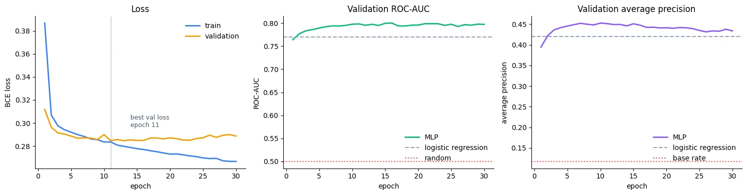
Best validation loss at epoch 11: 0.2846
Best validation ROC-AUC at epoch 16: 0.8000
Final epoch validation loss: 0.2887
Reading those curves
The left panel is the pattern to learn. Training loss falls steadily for all thirty epochs. Validation loss falls at first, reaches a minimum, and then turns upward while training loss continues to fall.
A useful mental model is:
training loss ↓ + validation loss ↓   → the model is improving on both seen and unseen data
training loss ↓ + validation loss ↑   → the model is improving on the training set but becoming worse on held-out data
That second pattern is evidence of overfitting. Overfitting means the model is becoming increasingly specialised to the training examples instead of improving its ability to generalise to new examples. It does not mean the model has literally memorised every row; it means the balance has shifted toward fitting training-specific detail that does not transfer as well.
It is mild here: the validation gap is not enormous and validation ROC-AUC stays roughly flat. But the direction is clear, and the thirty-epoch run was deliberately chosen so you could see the diagnosis.
We are not going to fix it yet. Dropout, weight decay, learning-rate schedules, and early stopping are Module 3 material. Today’s skill is recognising the pattern before applying a remedy.
Also notice that validation loss can degrade earlier or more clearly than validation ROC-AUC. Loss cares about the quality and confidence of the predicted probabilities. ROC-AUC only cares about the ordering of positive and negative examples. A model can therefore become increasingly overconfident while keeping a similar ranking. That distinction becomes important later when we discuss calibration.
final = evaluate(model, val_loader, loss_fn, DEVICE)print("VALIDATION RESULTS, after 30 epochs\n")print(f"{'model':<26}{'ROC-AUC':>10}{'avg prec':>11}{'train time':>13}")print("-" * 60)print(f"{'majority class':<26}{0.5:>10.4f}{y_val.mean():>11.4f}{'0.00s':>13}")print(f"{'logistic regression':<26}{logreg_auc:>10.4f}{logreg_ap:>11.4f}{logreg_time:>12.2f}s")print(f"{'MLP (50-64-32-1)':<26}{final['roc_auc']:>10.4f}" f"{final['avg_precision']:>11.4f}{train_time:>12.2f}s")print()print(f"MLP over logistic regression: " f"{final['roc_auc'] - logreg_auc:+.4f} ROC-AUC, " f"{final['avg_precision'] - logreg_ap:+.4f} average precision")print(f"Cost: {train_time / max(logreg_time, 1e-9):.0f}x the training time and " f"{count_params(model):,} parameters instead of {N_FEATURES + 1}.")VALIDATION RESULTS, after 30 epochs model ROC-AUC avg prec train time ------------------------------------------------------------ majority class 0.5000 0.1171 0.00s logistic regression 0.7699 0.4201 0.03s MLP (50-64-32-1) 0.7971 0.4338 6.24s MLP over logistic regression: +0.0272 ROC-AUC, +0.0137 average precision Cost: 224x the training time and 5,377 parameters instead of 51.
# What the model is worth in operational terms: precision-recall, not accuracy.prec, rec, thresholds = precision_recall_curve(final["labels"], final["probs"])lr_prec, lr_rec, _ = precision_recall_curve(y_val, logreg_probs)fig, axes = plt.subplots(1, 2, figsize=(12, 4.2))axes[0].plot(rec, prec, color="#8b5cf6", lw=2, label=f"MLP (AP={final['avg_precision']:.3f})")axes[0].plot(lr_rec, lr_prec, color="#94a3b8", lw=1.8, ls="--", label=f"logistic (AP={logreg_ap:.3f})")axes[0].axhline(y_val.mean(), color="#ef4444", ls=":", lw=1.5, label=f"base rate ({y_val.mean():.3f})")axes[0].set_xlabel("recall"); axes[0].set_ylabel("precision")axes[0].set_title("Precision–recall"); axes[0].legend(frameon=False)fpr, tpr, _ = roc_curve(final["labels"], final["probs"])lr_fpr, lr_tpr, _ = roc_curve(y_val, logreg_probs)axes[1].plot(fpr, tpr, color="#10b981", lw=2, label=f"MLP (AUC={final['roc_auc']:.3f})")axes[1].plot(lr_fpr, lr_tpr, color="#94a3b8", lw=1.8, ls="--", label=f"logistic (AUC={logreg_auc:.3f})")axes[1].plot([0, 1], [0, 1], color="#ef4444", ls=":", lw=1.5, label="random")axes[1].set_xlabel("false positive rate"); axes[1].set_ylabel("true positive rate")axes[1].set_title("ROC"); axes[1].legend(frameon=False, loc="lower right")for ax in axes: ax.spines[["top", "right"]].set_visible(False)plt.tight_layout()plt.show()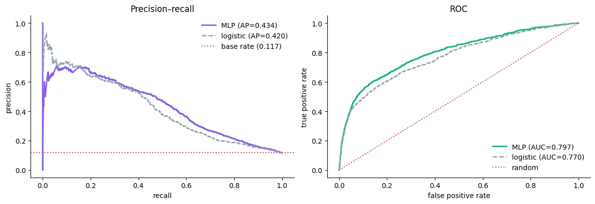
# Translate the curve into a business decision: who do we call?budget_fraction = 0.20 # we can afford to call 20% of the listk = int(len(final["probs"]) * budget_fraction)top_k = np.argsort(final["probs"])[::-1][:k]hits = final["labels"][top_k].sum()total_positives = final["labels"].sum()print(f"Suppose the call centre can contact {budget_fraction:.0%} of the list " f"({k:,} of {len(final['probs']):,} clients).\n")print(f" Calling at random : ~{int(k * y_val.mean()):,} subscribers reached " f"({y_val.mean():.1%} hit rate)")print(f" Calling the model's")print(f" highest-scoring {k:,} : {int(hits):,} subscribers reached " f"({hits / k:.1%} hit rate)")print(f"\n Lift: {(hits / k) / y_val.mean():.2f}x")print(f" Recall at 20% of budget: {hits / total_positives:.1%} of all " f"{int(total_positives):,} subscribers")Suppose the call centre can contact 20% of the list (1,356 of 6,782 clients). Calling at random : ~158 subscribers reached (11.7% hit rate) Calling the model's highest-scoring 1,356 : 481 subscribers reached (35.5% hit rate) Lift: 3.03x Recall at 20% of budget: 60.6% of all 794 subscribers
The verdict
The network beats logistic regression on the validation metrics shown above, but the margin is small relative to the additional model complexity and training cost. That is the fact to report; whether that trade-off is worthwhile is a deployment decision rather than a universal ML rule.
The operational question helps make the comparison concrete. Suppose a call centre can contact only a fixed fraction of the customer list. Then the practical task is often not:
“Can the model label every customer correctly at a chosen threshold?”
but:
“Can the model rank customers so that the limited call budget reaches more of the customers we care about?”
That distinction matters because ranking and classification are different tasks:
- classification: choose a threshold and turn each probability into a yes/no decision;
- ranking: sort customers from highest predicted risk to lowest and take the top
kbecause the team can only act onkcustomers.
For the latter task, average precision, ROC-AUC, and recall at a fixed capacity can be more informative than accuracy at an arbitrary threshold.
There is also a legitimate engineering trade-off around the logistic-regression baseline. Logistic regression is fast to train, its coefficients are comparatively easy to inspect, and it has fewer moving parts. An MLP adds nonlinear capacity, which may provide a measurable lift but also adds architecture, optimisation, checkpointing, and overfitting considerations.
The note therefore does not claim that the MLP should automatically be deployed. It shows what the experiment measured and gives you the evidence needed to discuss the trade-off.
The broader lesson is about tabular data. Here, the raw information has already been turned into a table of engineered numerical features. A representation is the numerical form in which information is presented to a model. On this dataset, much of the work of representing the customer has already been done by the preprocessing pipeline. Neural networks have a stronger automatic advantage on problems where the useful representation itself must be learned from less structured raw input, such as images, audio, or text.
Module 4 makes this comparison more rigorous, with gradient boosting as a third contender under a controlled experimental protocol. Today’s experiment is the mechanics-and-reasoning version that motivates that comparison.
-
At its best epoch the MLP reached an average precision well above what it shows in the final-epoch table, while its ROC-AUC barely moved between those two points. Given what each metric measures, what does that pattern say about which part of the ranking overfitting damaged first?
In the re-run, AP was 0.453 at epoch 10 but 0.434 at epoch 30, while ROC-AUC stayed ~0.797–0.798. ROC-AUC averages over all positive–negative pairs, dominated by the thousands of ordinary negatives; AP is driven by precision at the top of the list. So overfitting first damaged the ordering among the highest-scored customers (the model became overconfident about some of them), which is exactly the part of the ranking a call budget uses.
-
The lift calculation used the top 20% by predicted probability. Nothing in it required a threshold or a
predict()call. Why is ranking, rather than classification, the more useful framing for this problem?Because the business decision is "whom do we call first, given we can only call k people?". That is a ranking question. A threshold is an arbitrary line on probabilities that may not even be calibrated (class weighting shifts them, as Section 9 shows), and
predict()hides the ordering. Sorting by score and taking the top k maps directly onto capacity, and recall@k or lift are numbers a manager can act on. -
Argue the case for shipping logistic regression instead. What would have to be true about the business for that to be the better engineering decision?
Ship logistic regression if the extra lift isn't worth the extra cost and risk. The MLP adds ~0.03 AUC and ~0.01–0.03 AP, perhaps a dozen more subscribers per 1,356 calls. LR trains in 0.03 s vs ~6 s, has interpretable coefficients (often required in banking: you must explain why a customer was or wasn't contacted), gives well-calibrated probabilities, and has fewer failure modes to monitor and retrain. It's the right call when explainability or regulation matters, when the value per extra subscriber is small, or when the team can't support a neural pipeline. Measure in money: extra subscribers × value per subscriber vs engineering cost.
Why is logistic regression the important baseline here, rather than 'majority class'?
The majority baseline shows accuracy is misleading (88.3%, finds nobody). Logistic regression is the modelling reference that makes the MLP's result interpretable.
A call centre can phone 20% of customers. Which framing and metric fit best?
The team acts on the top k, so ordering matters, not a yes/no threshold. The MLP reached about 3× lift at 20% of the list.
Validation loss rises after epoch 11 while ROC-AUC stays roughly flat. What does that tell you?
- The model is overfitting mildly: it keeps fitting training-specific detail and becomes overconfident, which loss (which scores probability quality) penalises.
- ROC-AUC only cares about the ordering, which barely changed, so ranking quality held while calibration got worse.
Checkpointing that survives a crash
A checkpoint is a saved snapshot of training state. Saving only the model’s weights is enough to use the model for inference, but it is not enough to guarantee that you can continue training as if the interruption had never happened.
A resumable checkpoint here stores four essential pieces:
- model state: the learned weights and biases;
- optimizer state: information Adam has accumulated about the recent gradients and its update process;
- epoch: where training had reached;
- config: the settings needed to reconstruct the architecture and training setup, such as
hidden_sizes, input width, learning rate, and batch size.
Think of the distinction this way:
model weights     = what the network has learned
optimizer state   = what the optimizer remembers about how it has been learning
training position = where the run stopped
config            = how the model was constructed and trained
Save the state_dict, not the whole model object. Pickling the whole object ties the file to the Python class and module path used to create it; a refactor can therefore make an old pickled object difficult or impossible to load. A state dictionary stores the model state separately from the Python object definition, so the code can reconstruct the architecture explicitly.
What goes in a resumable checkpoint
What the network has learned: every weight and bias, keyed by module-tree path.
What Adam remembers: two running averages per parameter plus the step count.
Where training stopped, and the curves so far.
How to rebuild the architecture and training setup: in_features, hidden_sizes, lr, batch size, seed.
CONFIG = { "in_features": N_FEATURES, "hidden_sizes": (64, 32), "learning_rate": LEARNING_RATE, "batch_size": BATCH_SIZE, "seed": SEED,}def save_checkpoint(path, model, optimizer, epoch, history, config, extra=None): """Save everything needed to resume training into one file. Stores the model and optimizer state dicts, the epoch, the metric history, the configuration needed to rebuild the model, the PyTorch version and any extra values. Args: path: Destination file (e.g. ``checkpoints/bank_mlp.pt``). model: The model whose ``state_dict`` is saved. optimizer: The optimizer whose state (e.g. Adam's moment estimates) is saved. epoch: Number of epochs completed. history: Dict of per-epoch metrics. config: Dict with the architecture and training settings. extra: Optional dict of additional values to store, such as a validation score. Returns: The size of the saved file in bytes. """ torch.save({ "model_state_dict": model.state_dict(), "optimizer_state_dict": optimizer.state_dict(), "epoch": epoch, "history": history, "config": config, "torch_version": torch.__version__, **(extra or {}), }, path) return Path(path).stat().st_sizeckpt_path = CKPT_DIR / "bank_mlp.pt"size = save_checkpoint(ckpt_path, model, optimizer, EPOCHS, history, CONFIG, extra={"val_roc_auc": final["roc_auc"]})print(f"Saved {ckpt_path} ({size / 1024:.1f} KB)")print(f"\nWeights alone would be {count_params(model) * 4 / 1024:.1f} KB.")print("The file is larger because Adam's two moment buffers are one float per")print("parameter each — optimizer state roughly triples a checkpoint.")print("\nstate_dict keys (these are the module-tree paths from Section 2):")for k, v in list(model.state_dict().items()): print(f" {k:<26} {tuple(v.shape)}")Saved checkpoints/bank_mlp.pt (72.2 KB) Weights alone would be 21.0 KB. The file is larger because Adam's two moment buffers are one float per parameter each — optimizer state roughly triples a checkpoint. state_dict keys (these are the module-tree paths from Section 2): blocks.0.linear.weight (64, 50) blocks.0.linear.bias (64,) blocks.1.linear.weight (32, 64) blocks.1.linear.bias (32,) head.weight (1, 32) head.bias (1,)
def load_checkpoint(path, device): """Rebuild the model and optimizer from a checkpoint saved by ``save_checkpoint``. Reads the config to reconstruct ``BankMLP`` with the right widths, loads its weights, creates a fresh Adam optimizer and loads its saved state. Args: path: Checkpoint file to load. Only load files you trust: this uses ``weights_only=False``, which can execute pickled code. device: Device to place the restored model and optimizer state on. Returns: A tuple ``(model, optimizer, checkpoint_dict)``. """ ckpt = torch.load(path, map_location=device, weights_only=False) cfg = ckpt["config"] restored_model = BankMLP(cfg["in_features"], hidden_sizes=cfg["hidden_sizes"]).to(device) restored_model.load_state_dict(ckpt["model_state_dict"]) restored_opt = torch.optim.Adam(restored_model.parameters(), lr=cfg["learning_rate"]) restored_opt.load_state_dict(ckpt["optimizer_state_dict"]) return restored_model, restored_opt, ckptrestored, restored_opt, ckpt = load_checkpoint(ckpt_path, DEVICE)print(f"Restored from epoch {ckpt['epoch']}, " f"saved with torch {ckpt['torch_version']}")print(f"Recorded validation ROC-AUC: {ckpt['val_roc_auc']:.4f}")check = evaluate(restored, val_loader, loss_fn, DEVICE)print(f"\nRe-evaluated ROC-AUC : {check['roc_auc']:.4f}")print(f"Difference : {abs(check['roc_auc'] - final['roc_auc']):.2e}")assert np.allclose(check["probs"], final["probs"], atol=1e-6), "restored model must match"print("Restored model reproduces the original predictions exactly.")Restored from epoch 30, saved with torch 2.14.0 Recorded validation ROC-AUC: 0.7971 Re-evaluated ROC-AUC : 0.7971 Difference : 0.00e+00 Restored model reproduces the original predictions exactly.
# Does the optimizer state actually matter? Measure rather than assume.def resume_and_train(model_src, opt_state, n_epochs=3): """Continue training from saved weights, with or without the saved optimizer state. Used to measure how much restoring Adam's state matters: the same weights are resumed twice, once with the checkpointed optimizer state and once with a fresh optimizer. Args: model_src: Model whose weights are copied into a fresh ``BankMLP``. opt_state: An optimizer ``state_dict`` to load, or ``None`` for a fresh optimizer. n_epochs: Number of epochs to continue for. Returns: A list with the training loss of each resumed epoch. """ m = BankMLP(N_FEATURES, hidden_sizes=(64, 32)).to(DEVICE) m.load_state_dict(model_src.state_dict()) o = torch.optim.Adam(m.parameters(), lr=LEARNING_RATE) if opt_state is not None: o.load_state_dict(opt_state) losses = [] for _ in range(n_epochs): losses.append(train_one_epoch(m, train_loader, loss_fn, o, DEVICE)) return lossesseed_everything(SEED)with_state = resume_and_train(restored, ckpt["optimizer_state_dict"])seed_everything(SEED)without_state = resume_and_train(restored, None)print("Resuming for 3 epochs from the same weights:\n")print(f"{'epoch':>7}{'with optimizer state':>24}{'fresh optimizer':>19}{'difference':>14}")for i, (a, b) in enumerate(zip(with_state, without_state), start=1): print(f"{i:>7}{a:>24.5f}{b:>19.5f}{abs(a - b):>14.5f}")print()print("Barely any difference. That is the honest result on THIS problem, and it")print("is worth understanding rather than explaining away -- see the note below.")Resuming for 3 epochs from the same weights:
epoch with optimizer state fresh optimizer difference
1 0.26536 0.26541 0.00006
2 0.26425 0.26380 0.00045
3 0.26366 0.26323 0.00043
Barely any difference. That is the honest result on THIS problem, and it
is worth understanding rather than explaining away -- see the note below.
What that measurement actually showed
The two resumed runs are almost indistinguishable on this particular problem and for this short continuation. A fresh Adam loses its accumulated running statistics and starts those estimates again, but this small model sees 124 batches per epoch, so the new optimizer quickly rebuilds useful estimates.
That observation should not be turned into the rule “optimizer state does not matter.” The experiment only tells us what happened under these conditions. The optimizer state matters more when rebuilding it consumes a substantial fraction of the remaining training process, for example:
- resuming in the middle of an epoch or with only a few hundred optimisation steps left;
- fine-tuning, where the entire run may be short;
- using a learning-rate scheduler whose internal step position must also be restored;
- working with a large model where wasted steps are expensive.
The engineering conclusion is therefore about risk and reproducibility: save the optimizer state when you intend to resume training. The experiment is useful because it tells you that forgetting it may produce no obvious symptom on one small experiment — which is exactly why the bug can survive unnoticed.
weights_only=False above is required because this checkpoint contains ordinary Python dictionaries such as the config and history, not only tensors. Loading with that setting can unpickle Python objects, so only load checkpoints you produced yourself or otherwise trust. For a checkpoint that will be distributed, keep the serialised tensor state separate from trusted configuration data, as Lesson 2.4 does.
-
The checkpoint stores
hidden_sizesin its config. What breaks if you omit that information and later changeBankMLP’s default from(64, 32)to(128, 64)?load_checkpointrebuilds the model from the config. Withouthidden_sizesit would fall back on the class default, now(128, 64), while the saved tensors are shaped for(64, 32), soload_state_dictfails with size mismatch errors (e.g.blocks.0.linear.weight: copying (64, 50) … current model (128, 50)). Every old checkpoint becomes unloadable unless someone remembers the original architecture. The weights are meaningless without the recipe that built them. -
Adam keeps roughly two additional floating-point values per parameter for its moment estimates. For a 7-billion-parameter model, how large is that optimizer state in
float32, and what does that imply for fine-tuning on a single GPU?\(7\times10^9\) parameters × 2 moments × 4 bytes = 56 GB of Adam state. Add the float32 weights (28 GB) and gradients (28 GB) and you need about 112 GB before activations, more than one 80 GB GPU. Hence the tools of Modules 4 and 8: mixed precision / bf16 weights, 8-bit optimizers, sharding the state across GPUs (ZeRO/FSDP), and above all parameter-efficient fine-tuning (LoRA/QLoRA), where only a few million adapter parameters need optimizer state.
What four things make a checkpoint resumable?
The config (e.g. hidden_sizes) is needed to rebuild the architecture before loading the weights.
Resuming with a fresh Adam barely changed this run. The right conclusion is…
One small experiment does not make a rule. The engineering conclusion is about risk and reproducibility.
Adam keeps about two extra floats per parameter. Estimate the optimizer state for a 7-billion-parameter model in float32 and what that implies.
- 7B × 2 × 4 bytes ≈ 56 GB of optimizer state, on top of the weights (≈ 28 GB) and gradients (≈ 28 GB).
- Full fine-tuning of such a model does not fit on a single typical GPU, which motivates parameter-efficient methods (LoRA, Module 8) and memory tricks (Module 4).
Now modify the loop yourself
Module 2’s end-of-module competency is building a neural network and writing or modifying its training loop. Running someone else’s loop is not the same skill.
The three modifications below are deliberately small. Each one changes one part of the experiment while leaving the rest of the training mechanism recognisable.
Modification 1: weight the positive class
BCEWithLogitsLoss(pos_weight=w) changes the training objective by multiplying the loss contribution from positive examples by w. With an 11.7% positive rate, the natural demonstration value is the ratio of negative examples to positive examples.
The important conceptual distinction is that changing the training objective is not the same thing as changing the decision threshold later. We will measure both the ranking and the threshold-based behaviour so you can see the difference rather than relying on a slogan.
pos_weight_value = (1 - y_train.mean()) / y_train.mean()print(f"negatives per positive: {pos_weight_value:.2f}")def run_experiment(pos_weight=None, epochs=15, label=""): """Train a fresh ``BankMLP`` with an optionally class-weighted loss, then evaluate it. The training loss can up-weight positive examples via ``pos_weight``; evaluation always uses the *unweighted* loss so the two runs are compared on the same scale. Args: pos_weight: Multiplier for positive examples' loss (e.g. negatives ÷ positives), or ``None`` for an unweighted loss. epochs: Number of training epochs. label: Name for the run (for your own bookkeeping). Returns: A tuple ``(model, results)`` where ``results`` is the dict from ``evaluate``. """ seed_everything(SEED) m = BankMLP(N_FEATURES, hidden_sizes=(64, 32)).to(DEVICE) o = torch.optim.Adam(m.parameters(), lr=LEARNING_RATE) lf = nn.BCEWithLogitsLoss( pos_weight=torch.tensor([pos_weight], dtype=torch.float32, device=DEVICE) if pos_weight else None) eval_fn = nn.BCEWithLogitsLoss() # evaluate on the UNWEIGHTED loss, always for _ in range(epochs): train_one_epoch(m, train_loader, lf, o, DEVICE) return m, evaluate(m, val_loader, eval_fn, DEVICE)m_plain, r_plain = run_experiment(None, 15, "unweighted")m_weighted, r_weighted = run_experiment(pos_weight_value, 15, "weighted")print(f"\n{'run':<22}{'ROC-AUC':>10}{'avg prec':>11}{'mean P(yes)':>14}")print("-" * 57)print(f"{'unweighted':<22}{r_plain['roc_auc']:>10.4f}" f"{r_plain['avg_precision']:>11.4f}{r_plain['probs'].mean():>14.4f}")print(f"{'pos_weight=' + f'{pos_weight_value:.1f}':<22}{r_weighted['roc_auc']:>10.4f}" f"{r_weighted['avg_precision']:>11.4f}{r_weighted['probs'].mean():>14.4f}")print(f"\nActual positive rate: {y_val.mean():.4f}")negatives per positive: 7.55 run ROC-AUC avg prec mean P(yes) --------------------------------------------------------- unweighted 0.7968 0.4464 0.1080 pos_weight=7.5 0.7989 0.4478 0.3620 Actual positive rate: 0.1171
# Where the weighting actually changes behaviour: the default 0.5 threshold.print(f"{'run':<22}{'precision':>11}{'recall':>10}{'F1':>8} (threshold 0.5)")print("-" * 53)for name, res in [("unweighted", r_plain), ("weighted", r_weighted)]: pred = (res["probs"] >= 0.5).astype(int) tn, fp, fn_, tp = confusion_matrix(res["labels"], pred).ravel() precision = tp / max(tp + fp, 1) recall = tp / max(tp + fn_, 1) f1 = f1_score(res["labels"], pred) print(f"{name:<22}{precision:>11.4f}{recall:>10.4f}{f1:>8.4f}")fig, ax = plt.subplots(figsize=(8, 3.5))bins = np.linspace(0, 1, 41)ax.hist(r_plain["probs"], bins=bins, alpha=0.6, label="unweighted", color="#3b82f6")ax.hist(r_weighted["probs"], bins=bins, alpha=0.6, label="pos_weight", color="#f59e0b")ax.axvline(0.5, color="#64748b", ls=":", lw=1.5)ax.set_xlabel("predicted P(subscribe)"); ax.set_ylabel("count")ax.set_yscale("log")ax.set_title("Class weighting moves the probabilities, not the ranking")ax.legend(frameon=False)ax.spines[["top", "right"]].set_visible(False)plt.tight_layout()plt.show()run precision recall F1 (threshold 0.5) ----------------------------------------------------- unweighted 0.6553 0.2418 0.3533 weighted 0.3318 0.6398 0.4370
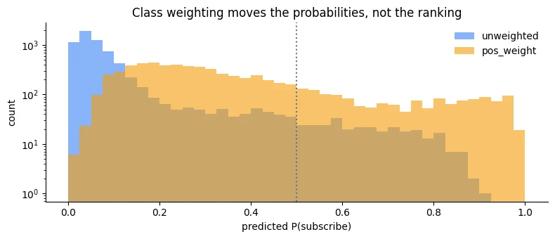
This is the result worth understanding, because it separates two effects that are often mixed together.
Class weighting changed the training objective: positive examples counted more heavily when the model learned. In this experiment it barely moved ROC-AUC or average precision, which are primarily measures of ranking. What changed substantially was the distribution of predicted probabilities and therefore the behaviour of the default 0.5 threshold: recall increased while precision decreased.
An operating point is simply the particular decision rule you choose after the model has produced scores. For example:
probability >= 0.50  → act
probability <  0.50  → do not act
Changing that threshold moves you to a different precision/recall trade-off without retraining the model.
The weighted model in this experiment is also less calibrated. Calibration asks whether predicted probabilities correspond to observed frequencies. For example, among cases assigned approximately 0.70 probability, a well-calibrated model would have an observed positive rate near 70% over a large enough group. A model can preserve its ranking while its probability scale becomes poorly calibrated.
So the practical distinction is:
- loss weighting: change what the model is encouraged to care about while learning;
- threshold selection: change which scores are converted into actions after the model is trained.
They can sometimes lead to similar precision/recall trade-offs, but they are not the same intervention and they have different effects on the learned scores and calibration.
Choose deliberately based on the objective you are trying to optimise.
Modification 2: add a metric to the loop
Adding a per-epoch metric is a small code change, but it teaches an important general pattern: a training loop can record quantities that describe both optimisation behaviour and the business-facing outcome you actually care about.
def train_with_extra_metric(model, epochs=15): """The training loop plus two extra measurements recorded every epoch. Logs the total gradient norm on each epoch's first batch (a view of how training is converging) and recall when only the top 20% of validation customers can be called (a metric the business recognises), alongside average precision. Args: model: The model to train. epochs: Number of epochs. Returns: A dict of per-epoch lists: ``"val_ap"``, ``"recall_at_20pct"`` and ``"grad_norm"``. """ optimizer = torch.optim.Adam(model.parameters(), lr=LEARNING_RATE) lf = nn.BCEWithLogitsLoss() log = {"val_ap": [], "recall_at_20pct": [], "grad_norm": []} for _ in range(epochs): # --- the extra: capture gradient norm on the first batch of each epoch --- model.train() first = True for xb, yb in train_loader: xb, yb = xb.to(DEVICE), yb.to(DEVICE) optimizer.zero_grad() loss = lf(model(xb), yb) loss.backward() if first: total_norm = torch.sqrt(sum((p.grad ** 2).sum() for p in model.parameters())) log["grad_norm"].append(total_norm.item()) first = False optimizer.step() res = evaluate(model, val_loader, lf, DEVICE) k = int(len(res["probs"]) * 0.20) top = np.argsort(res["probs"])[::-1][:k] log["val_ap"].append(res["avg_precision"]) log["recall_at_20pct"].append(res["labels"][top].sum() / res["labels"].sum()) return logseed_everything(SEED)m_metric = BankMLP(N_FEATURES, hidden_sizes=(64, 32)).to(DEVICE)log = train_with_extra_metric(m_metric, epochs=15)fig, axes = plt.subplots(1, 2, figsize=(12, 3.8))axes[0].plot(range(1, 16), log["recall_at_20pct"], color="#8b5cf6", lw=2, marker="o", ms=4)axes[0].set_xlabel("epoch"); axes[0].set_ylabel("recall @ 20% budget")axes[0].set_title("A metric the business would recognise")axes[1].plot(range(1, 16), log["grad_norm"], color="#ef4444", lw=2, marker="o", ms=4)axes[1].set_xlabel("epoch"); axes[1].set_ylabel("gradient L2 norm")axes[1].set_title("Gradient norm, first batch of each epoch")for ax in axes: ax.spines[["top", "right"]].set_visible(False)plt.tight_layout()plt.show()print(f"recall@20%: {log['recall_at_20pct'][0]:.3f} (epoch 1) " f"-> {log['recall_at_20pct'][-1]:.3f} (epoch 15)")print(f"grad norm : {log['grad_norm'][0]:.4f} (epoch 1) " f"-> {log['grad_norm'][-1]:.4f} (epoch 15)")print("\nGradient norm shrinking as training proceeds is what convergence looks like.")print("A norm that grows without bound is an exploding gradient. Day 3 covers both.")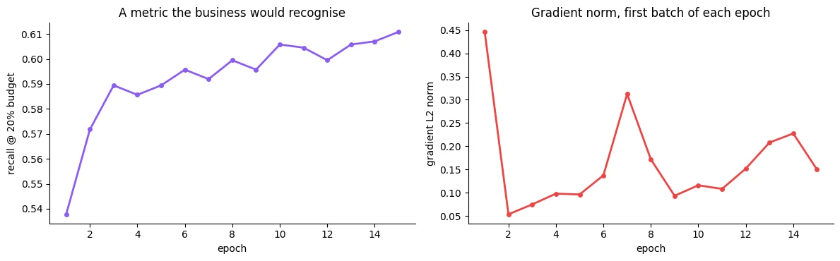
recall@20%: 0.538 (epoch 1) -> 0.611 (epoch 15)
grad norm : 0.4461 (epoch 1) -> 0.1499 (epoch 15)

Gradient norm shrinking as training proceeds is what convergence looks like.
A norm that grows without bound is an exploding gradient. Day 3 covers both.
Modification 3: early stopping, written by hand
Section 7 showed validation loss bottoming out in the low teens and drifting upward for the remaining two-thirds of the run. Early stopping keeps the best model and stops paying for epochs that make things worse.
Writing it yourself once — rather than importing a callback — makes the mechanism concrete: track the best score, count epochs since it improved, keep a copy of the winning weights.
def train_with_early_stopping(max_epochs=60, patience=5, min_delta=1e-4): """Train until validation loss stops improving, then restore the best weights. After each epoch the validation loss is compared with the best so far; only an improvement larger than ``min_delta`` resets the patience counter. Training stops after ``patience`` epochs without improvement. Args: max_epochs: Upper limit on training epochs. patience: Epochs without meaningful improvement before stopping. min_delta: Smallest decrease in validation loss that counts as improvement. Returns: A tuple ``(model, best_epoch, best_loss, curve)``: the model with its best weights restored, the epoch they came from, that epoch's validation loss, and the list of validation losses for every epoch that ran. """ seed_everything(SEED) m = BankMLP(N_FEATURES, hidden_sizes=(64, 32)).to(DEVICE) o = torch.optim.Adam(m.parameters(), lr=LEARNING_RATE) lf = nn.BCEWithLogitsLoss() best_loss = float("inf") best_epoch = 0 best_weights = None epochs_without_improvement = 0 curve = [] for epoch in range(1, max_epochs + 1): train_one_epoch(m, train_loader, lf, o, DEVICE) res = evaluate(m, val_loader, lf, DEVICE) curve.append(res["loss"]) if res["loss"] < best_loss - min_delta: best_loss = res["loss"] best_epoch = epoch best_weights = copy.deepcopy(m.state_dict()) # deepcopy: state_dict shares storage epochs_without_improvement = 0 else: epochs_without_improvement += 1 if epochs_without_improvement >= patience: print(f"Stopped at epoch {epoch}: no improvement for {patience} epochs.") break else: print(f"Ran the full {max_epochs} epochs without triggering.") m.load_state_dict(best_weights) # restore the best, not the last return m, best_epoch, best_loss, curvebest_model, best_epoch, best_loss, curve = train_with_early_stopping()print(f"Best epoch {best_epoch}, validation loss {best_loss:.4f}")print(f"Epochs actually run: {len(curve)} (of a 60 budget)")es_result = evaluate(best_model, val_loader, nn.BCEWithLogitsLoss(), DEVICE)print(f"\n{'model':<32}{'val loss':>10}{'ROC-AUC':>10}{'avg prec':>11}")print("-" * 63)print(f"{'30 epochs, last weights':<32}{history['val_loss'][-1]:>10.4f}" f"{final['roc_auc']:>10.4f}{final['avg_precision']:>11.4f}")print(f"{f'early stopped, best (ep {best_epoch})':<32}{best_loss:>10.4f}" f"{es_result['roc_auc']:>10.4f}{es_result['avg_precision']:>11.4f}")Track the best validation loss, count epochs without real improvement, stop when patience runs out, and restore the best weights.
- 1
Only an improvement larger than
min_deltacounts, so floating-point jitter can't reset the counter. - 2
state_dict()returns references to the live tensors, so withoutdeepcopyyour 'best' snapshot would keep changing. - 3
Patience exhausted: stop paying for epochs that make things worse.
- 4
Restore the best weights, not the last ones.
Stopped at epoch 16: no improvement for 5 epochs.
Best epoch 11, validation loss 0.2846
Epochs actually run: 16 (of a 60 budget)

model                             val loss   ROC-AUC   avg prec
---------------------------------------------------------------
30 epochs, last weights             0.2887    0.7971     0.4338
early stopped, best (ep 11)         0.2846    0.7982     0.4515
fig, ax = plt.subplots(figsize=(9, 4))ax.plot(range(1, len(curve) + 1), curve, color="#f59e0b", lw=2, label="validation loss")ax.scatter([best_epoch], [best_loss], color="#10b981", s=90, zorder=5, label=f"best (epoch {best_epoch})")ax.axvspan(best_epoch, len(curve), alpha=0.10, color="#ef4444")ax.text(best_epoch + 0.3, max(curve) * 0.999, f"{len(curve) - best_epoch} epochs of patience,\nthen stop", fontsize=9, color="#7f1d1d", va="top")ax.set_xlabel("epoch"); ax.set_ylabel("validation BCE loss")ax.set_title("Early stopping: keep the best weights, not the last")ax.legend(frameon=False)ax.spines[["top", "right"]].set_visible(False)plt.tight_layout()plt.show()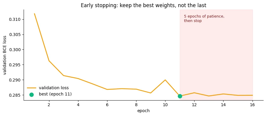
Two details in that implementation are load-bearing.
copy.deepcopy(m.state_dict()) is necessary because the tensors returned by state_dict() refer to the model’s current underlying storage. If you merely keep the dictionary and continue training, the live model keeps changing the values those references point to. Your supposed “best weights” can therefore silently become the latest weights.
deepcopy creates independent copies of the state tensors. Now the snapshot really is a snapshot, so load_state_dict(best_weights) can restore the model to the parameter values that produced the best validation loss.
min_delta defines what counts as a meaningful improvement. Without it, tiny floating-point changes can repeatedly reset the patience counter even when the validation loss is effectively unchanged.
Patience is the number of consecutive epochs you are willing to wait without meaningful improvement before stopping. Early stopping therefore has two jobs: identify the best validation point seen so far, and stop spending computation after the model has failed to improve for long enough.
Note the honest caveat. Early stopping chooses an epoch by looking at the validation set. That means the selected validation score is mildly optimistic because you chose the best result among many measurements on the same set. This is why a separate test set exists and why we have not used ours to choose the stopping point. Module 4 treats this issue more formally.
Your turn
Three exercises, in increasing difficulty. Each is a modification to code above, not a rewrite.
- Track precision at a fixed recall. Add a metric to
train_with_extra_metricthat reports precision at the threshold where recall first reaches 0.50. Which epoch is best by that measure, and is it the same epoch that minimises validation loss? Explain why the two criteria can disagree. - Make the width configurable and sweep it.
BankMLPalready acceptshidden_sizes. Train(16,),(64, 32)and(256, 128, 64)for fifteen epochs each, and plot validation average precision against parameter count. Does more capacity help on this dataset? Predict first, then measure. - Early stopping on the right quantity. The implementation above monitors validation loss. Rewrite it to monitor average precision instead — note that the comparison direction flips because higher average precision is better. Do the two criteria choose the same epoch? If not, explain the difference in terms of what each quantity measures and the business objective you established earlier.
pos_weight=7.5 barely moved ROC-AUC but recall at threshold 0.5 jumped from 0.24 to 0.64. Why?
Loss weighting changes what the model cares about while learning; threshold choice changes which scores become actions. The weighted model is also less calibrated.
Why copy.deepcopy(model.state_dict()) when saving the best weights for early stopping?
Without an independent copy, the snapshot silently becomes the latest weights.
Why is the validation score chosen by early stopping mildly optimistic, and what protects you?
- You pick the best of many measurements on the same validation set, so the chosen score benefits from luck on that set.
- A separate test set, never used to make choices, gives the honest final estimate.
Conclusion
You built an MLP, trained it with a loop you wrote, and evaluated it against baselines that make the result contestable rather than automatic. The main lesson is not a collection of API calls. It is understanding what each piece of the training system is responsible for.
On nn.Module. A PyTorch module is both the place where you define the forward computation and the structure PyTorch uses to register child modules and parameters. Registration is what lets optimizers find trainable tensors, device movement reach the model’s state, checkpoints collect that state, and mode changes propagate through the module tree. A layer hidden inside a plain Python list is not automatically registered.
On shapes. A shape is the size of a tensor along each dimension. Dry-run a fake batch before real data touches the model. Forward hooks let you inspect intermediate inputs and outputs when one shape check is not enough. Both techniques are cheap debugging tools because they test the model’s wiring independently of the dataset.
On the output head. For binary classification you can use one raw logit with BCEWithLogitsLoss or two class logits with CrossEntropyLoss. Both are valid. The important rule is to match the output representation, label format, and loss function. When the loss expects logits, do not add a sigmoid or softmax to forward just to obtain probabilities during training.
On the loop. The core sequence is:
clear old gradients
        ↓
forward pass
        ↓
calculate loss
        ↓
backward pass → gradients
        ↓
optimizer step → updated parameters
The surrounding bookkeeping matters just as much: accumulate loss.item(), weight batch means by actual batch size when calculating a dataset-level mean, and make the training/evaluation mode explicit.
On eval() and no_grad(). They solve different problems. eval() changes the behaviour of modules that have training/evaluation modes. no_grad() prevents PyTorch from building a gradient graph when gradients are not needed. A correct validation pass normally uses both.
On the result. The MLP produced a measurable validation improvement over logistic regression in this experiment, but the margin was small compared with the additional machinery. Whether that trade-off is worthwhile depends on the deployment requirements. The experiment therefore informs an engineering decision; it does not make that decision for you.
On ranking. A probability model can be used in two different ways: choose a threshold and classify everyone, or sort everyone by score and act on the highest-ranked cases. When operational capacity is limited, ranking can be the more direct representation of the problem. That is why ROC-AUC, average precision, and recall at a fixed budget appear alongside threshold-based metrics.
On the curves. Validation loss eventually turned upward while training loss continued downward. That is the observable pattern of overfitting: optimisation on the training set continues while held-out performance stops improving. We deliberately diagnosed it before applying a remedy.
On modification. You changed the class weighting, observed how it affected the score distribution and threshold behaviour, added metrics and a gradient-norm probe, and implemented early stopping yourself. You also saw why a best-weight snapshot must be a real copy and why a resumable checkpoint needs more than the model weights.
If you can explain these mechanisms rather than merely reproduce the code, you are no longer just running a training loop — you understand enough of it to modify and defend it.
Transition to Lesson 2.4
Everything above lives in a notebook. Notebooks are excellent for the exploratory work you have just done — inspecting tensors, plotting curves, changing one thing, and rerunning cells. They become less suitable when you need a repeatable software artifact.
The problem is execution state: notebook cells can be run out of order, the exact settings used for an experiment can be hidden in earlier cells, and another program cannot cleanly import a single part of the notebook. Reproducing an experiment therefore becomes harder as the project grows.
Lesson 2.4 fixes this by moving the same ideas into a normal project structure. Its cells write real files — src/data/, src/models/, src/training/, configs/, a README.md, and a .gitignore — and its final section runs the training from the command line:
python -m src.training.train --config configs/baseline.yaml
The goal is not to abandon notebooks. It is to move the code that should be reusable, testable, reviewable, and repeatable into a project structure while keeping notebooks available for exploration.
Lesson 2.4 also covers environment and dependency pinning so the software versions are explicit, and Git practices so changes can be reviewed. The project skeleton is the same structure Module 10 requires for the final portfolio artifact.
Wrap-up
nn.Moduleregisters layers assigned as attributes (and insidenn.ModuleList/ModuleDict). Layers in plain lists are invisible toparameters(), so they're silently never trained. Assert the parameter count.- Call
model(x), nevermodel.forward(x): hooks run only through__call__. - Compose models from blocks; use a custom
forwardwhenever data flow isn't a straight chain. - Dry-run a fake batch and trace shapes with forward hooks before using real data. Remove hooks afterwards.
- Output logits; let
BCEWithLogitsLoss/CrossEntropyLossapply sigmoid/softmax stably. Never add a sigmoid inforwardas well. - Bookkeeping:
zero_grad()every step, accumulateloss.item() × batch size, divide by examples seen. - Validation needs both
model.eval()(layer behaviour) andtorch.no_grad()(no graph); compute metrics once over all predictions. - Judge a model against baselines. Here the MLP beats logistic regression by ~0.03 AUC at 200× the cost; ranking metrics and recall@budget match the business question.
- Checkpoints hold model state, optimizer state, epoch and config; load untrusted files only with
weights_only=True. - Class weighting changes probabilities and the operating point, not the ranking. Early stopping keeps the best weights (use
deepcopy).
Quick check
You store three layers in self.layers = [nn.Linear(8, 8), ...] (a plain list). What happens when you train?
Plain lists aren't registered, so model.parameters() never yields them and the optimizer can't update them. No error is raised.
BankMLP(50, hidden_sizes=(64, 32)) has how many parameters?
(50×64+64) + (64×32+32) + (32×1+1) = 3,264 + 2,080 + 33 = 5,377.
Why does BCEWithLogitsLoss take logits rather than probabilities?
Sigmoid-then-log breaks in floating point for confident predictions; the fused form stays proportional to the error.
What does model.eval() change?
eval() is about layer behaviour; no_grad() is about the graph. You need both for validation.
A call centre can phone 20% of customers. Which evaluation fits best?
The decision is whom to call first. Rank by score and measure what the top 20% captures.
Why copy.deepcopy(model.state_dict()) when saving the best weights during early stopping?
Without a real copy, your 'best' snapshot silently becomes the latest weights.
Questions and discussion
Ask about this lesson, share what you found in a lab, or help someone else. Posts are public on the course's GitHub Discussions: anyone can read them, and you need a GitHub account to post.
Opening it loads giscus from giscus.app.