How Neural Networks Learn from Text
Classroom material
- Time
- ~51 min
- Sections
- 12
- Code cells
- 22
- Figures
- 7
Before you start
How can a network turn words, which are just symbols, into numbers that capture meaning?
- You will be able to
- explain why raw text cannot be fed to a network, and what tokenisation does;
- build a vocabulary and convert text into token IDs;
- explain why one-hot vectors cannot express similarity, and how embedding layers fix this;
- measure similarity between words with cosine similarity;
- train embeddings with two different objectives and explain, with measurements, why they learn different things;
- explain the difference between static and contextual representations.
In Lessons 5.1 and 5.2, our raw data was already made of numbers: every pixel had a brightness between 0 and 255. The challenge was turning those numbers into a useful description.
Text starts one step further back. A sentence is a sequence of symbols (letters, spaces, punctuation), and a neural network cannot multiply a weight by the letter "g". So before a network can learn anything from text, we must answer a more basic question: how do we turn words into numbers at all? And then: how do we make those numbers meaningful, so that "great" and "excellent" end up close together and "great" and "terrible" do not?
The answer is the embedding: a learned vector of numbers for each word. Embeddings are one of the most important ideas in modern AI. Every language model, every semantic search engine and every chatbot begins by turning text into embeddings. In this lesson we build them from the ground up, train them two different ways, and discover something important: an embedding learns whatever its training objective rewards.
Key question: How can a network turn words, which are just symbols, into numbers that capture meaning?
Prerequisites
read Lessons 5.1 and 5.2. You should be comfortable with PyTorch tensors and shapes, nn.Module, and the training loop.
Setup — imports, versions and device detection used by the notebook (1 cells)
Run this cell first. Alongside PyTorch, we use pandas to load the dataset and Python's built-in re (regular expressions) and collections modules to process text.
Environment and results. The saved outputs record one CPU reference run; random seeds reduce variation but do not guarantee identical numbers across computers. Read the comparisons as evidence from that run. Training times depend on your hardware.
If packages are missing, install them into your notebook environment, then restart the kernel and run from the beginning:
%pip install torch==2.14.1 numpy==2.5.4 pandas==3.0.6 matplotlib==3.11.2 scikit-learn==1.9.1 scipy==1.18.1
import os, re, collections, urllib.requestimport numpy as npimport pandas as pdimport torchimport torch.nn as nnimport torch.nn.functional as Fimport matplotlib.pyplot as plttorch.manual_seed(0)np.random.seed(0)device = "cuda" if torch.cuda.is_available() else "cpu"print("PyTorch", torch.__version__, "| device:", device)PyTorch 2.14.1 | device: cpu
The Big Picture: From Text to Numerical Representations
Here is the whole journey a piece of text takes before a network can learn from it. Every later section explains one step of it.
- Raw text:
"This movie wasn't GOOD.<br />It was great!" - Tokenisation: split the text into units called tokens, here words:
this,movie,wasn't,good,it,was,great. - Token IDs: look each token up in a fixed vocabulary (a numbered list of all known tokens) and replace it with its number.
- Embeddings: replace each ID with a learned vector, for example 32 numbers per word. Similar words should get similar vectors.
- Model: combine the vectors and make a prediction, for example "positive review".
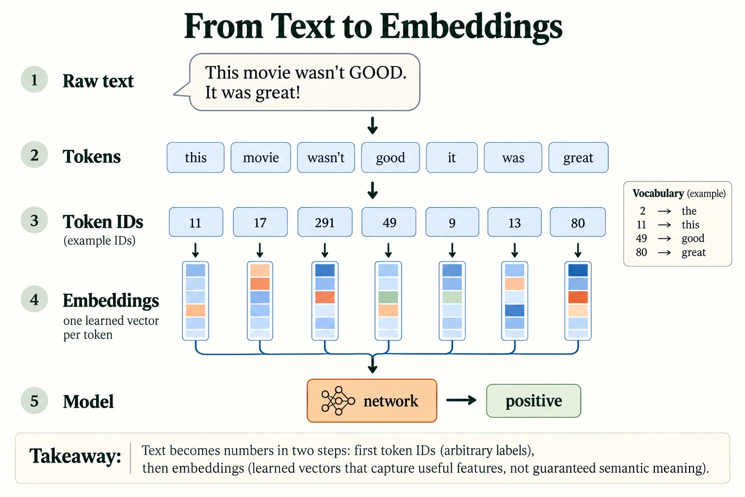
Figure 5.3.1. Token IDs are arbitrary vocabulary indices. An embedding lookup turns each index into a learned vector. The displayed IDs are an example vocabulary, not the recorded IDs of this experiment.
The first three steps are fixed preprocessing. Step 4 is where the learning happens, and it is the focus of this lesson.
We will work with IMDb movie reviews: 50,000 reviews from the Internet Movie Database, each labelled positive or negative. It is one of the most widely used datasets for learning about text, and we will return to it in Modules 7 and 8. The download happens only the first time you run the cell.
URL = "https://raw.githubusercontent.com/Ankit152/IMDB-sentiment-analysis/master/IMDB-Dataset.csv"PATH = "data/imdb/IMDB-Dataset.csv"os.makedirs("data/imdb", exist_ok=True)if not os.path.exists(PATH): urllib.request.urlretrieve(URL, PATH)print(f"file size: {os.path.getsize(PATH) / 1e6:.0f} MB")df = pd.read_csv(PATH)print("rows:", len(df), "| columns:", list(df.columns))print("exact duplicate rows:", df.duplicated().sum())df = df.drop_duplicates().sample(frac=1, random_state=0).reset_index(drop=True) # remove duplicates, shuffleprint("rows after removing duplicates:", len(df))print(df.sentiment.value_counts().to_dict())file size: 66 MB
rows: 50000 | columns: ['review', 'sentiment']
exact duplicate rows: 418
rows after removing duplicates: 49582
{'positive': 24884, 'negative': 24698}
The file has 50,000 rows with two columns, review and sentiment. But 418 rows are exact duplicates: the same review text with the same label, appearing more than once. Duplicates are dangerous: if one copy lands in the training set and another in the validation set, the model is tested on a review it has already seen, and its score looks better than it really is. So we remove them, leaving 49,582 reviews (24,884 positive and 24,698 negative, almost perfectly balanced), and shuffle the order.
Common mistake: splitting a dataset into training and validation sets before removing duplicates. Copies of the same example then end up on both sides of the split, and validation accuracy is inflated. Deduplicate first, then split. You will meet this issue again, in more depth, in Module 8.
To keep this notebook fast, we use 20,000 reviews for training and 5,000 for validation. Here is the start of the first training review:
train_df, val_df = df.iloc[:20000], df.iloc[20000:25000]print("train:", len(train_df), "| validation:", len(val_df))review = train_df.review.iloc[0]print(review[:400])train: 20000 | validation: 5000 Originally I was a Tenacious D fan of their first album and naturally listened to a few tracks off The P.O.D. and was rather disappointed. After watching the movie, my view was changed. The movie is pretty funny from beginning to the end and found my self engaged in it even though it was really was a stupid storyline because of the attitudes that KG and Jaybles portray in the movie. <br /><br />Mu
Which step makes token vectors learn useful task information?
Training the embedding parameters through an objective.
Why Neural Networks Cannot Process Raw Text Directly
Look closely at that review and think about it from a network's point of view. Three problems stand out.
Problem 1: text is made of symbols, not numbers. A network can only do arithmetic. Every character does have a numeric code (its Unicode code point), but those codes are arbitrary labels.
words_per_review = train_df.review.str.split().str.len()print("words per review: min", words_per_review.min(), "| median", int(words_per_review.median()), "| max", words_per_review.max())print("first 12 characters as code points:", [ord(c) for c in review[:12]])words per review: min 10 | median 173 | max 2470 first 12 characters as code points: [79, 114, 105, 103, 105, 110, 97, 108, 108, 121, 32, 73]
The capital O that begins the review is stored as 79 and the r after it as 114. Nothing about 79 or 114 relates to meaning. By that numbering, "good" and "food" differ by one letter and would look almost identical, while "good" and "great" would look quite different. Arithmetic on character codes is arithmetic on spelling, not meaning.
Problem 2: texts have different lengths. The shortest training review has 10 words, the median has 173 and the longest has 2,470. But the networks you have built expect inputs of a fixed shape, such as a batch of shape (64, 784). Text needs a way to be cut and padded to a common shape.
Problem 3: the same meaning can be written in many ways. "GOOD", "Good" and "good." are the same word to a reader but different strings to a computer. The review also contains HTML line-break tags, <br />, left over from the web page it was copied from.
The rest of this lesson solves these problems one at a time: tokenisation deals with Problem 3 and prepares for Problem 1; token IDs and embeddings solve Problem 1; padding and truncation solve Problem 2.
-
Why would it be a poor idea to represent each word by the sum of its characters' code points?
The sum of code points depends only on spelling, and different words can share the same sum: "dog" and "god" have identical letters, so identical sums, but very different meanings. And words with similar meanings ("good", "great") would get unrelated sums. The number would carry no information about meaning.
Why are character codes poor semantic measurements?
Their numerical relationships encode symbols, not semantic similarity.
Tokenisation and Token IDs
3.1 Splitting text into tokens
Tokenisation means splitting text into the units the model will treat as its basic building blocks: the tokens. The simplest idea, splitting on spaces, already runs into trouble:
def tokenize(text): """Lowercase, remove the stated HTML breaks and extract letter/apostrophe tokens. Arguments: text: Input text string. """ text = text.lower().replace("<br />", " ") return re.findall(r"[a-z']+", text)sentence = "This movie wasn't GOOD.<br /><br />It was great!"print("split on spaces:", sentence.split())print("our tokenizer: ", tokenize(sentence))split on spaces: ['This', 'movie', "wasn't", 'GOOD.<br', '/><br', '/>It', 'was', 'great!'] our tokenizer: ['this', 'movie', "wasn't", 'good', 'it', 'was', 'great']
Splitting on spaces produces tokens such as 'GOOD.<br' and '/>It', which mix words with punctuation and HTML. Our small tokenize function does three things instead: it lowercases the text, removes the <br /> tags, and keeps only runs of letters and apostrophes. The result, ['this', 'movie', "wasn't", 'good', 'it', 'was', 'great'], is much cleaner.
Every tokeniser involves choices like these, and they matter. Lowercasing means "Apple" (the company) and "apple" (the fruit) become the same token. Dropping punctuation throws away the difference between "great!" and "great?". There is no perfect tokeniser, only one that suits the task. In this lesson we use whole words. In Module 6 you will meet subword tokenisers, which split rare words into common pieces, and which are widely used by modern language models.
3.2 Building a vocabulary
Next we tokenise all 20,000 training reviews and count how often each word appears.
train_tokens = [tokenize(t) for t in train_df.review]val_tokens = [tokenize(t) for t in val_df.review]counts = collections.Counter(w for doc in train_tokens for w in doc)total = sum(counts.values())print("tokens in training reviews:", total)print("distinct words:", len(counts))for n in [1000, 10000]: covered = sum(c for _, c in counts.most_common(n)) / total print(f"the {n} most common words cover {covered:.1%} of all tokens")print("10 most common:", [w for w, _ in counts.most_common(10)])tokens in training reviews: 4617067 distinct words: 79754 the 1000 most common words cover 76.3% of all tokens the 10000 most common words cover 94.3% of all tokens 10 most common: ['the', 'and', 'a', 'of', 'to', 'is', 'in', 'it', 'i', 'this']
The training reviews contain 4,617,067 tokens but only 79,754 distinct words. The counts are extremely uneven: the 1,000 most common words cover 76.3% of all the tokens, and the 10,000 most common cover 94.3%. The most common words are tiny "function words" such as the, and, a and of.
The plot below shows this unevenness. Each point is one word, ranked from most common to least common, plotted against how often it occurs. Both axes are logarithmic (each step is a factor of 10).
freqs = np.array(sorted(counts.values(), reverse=True))plt.figure(figsize=(6, 3.8))plt.loglog(np.arange(1, len(freqs) + 1), freqs)plt.axvline(10000, color="grey", ls="--", lw=1, label="vocabulary cut-off (10,000 words)")plt.xlabel("word rank (1 = most common)"); plt.ylabel("number of occurrences")plt.title("A few words are very common; most words are rare"); plt.legend(); plt.grid(alpha=0.3)plt.tight_layout(); plt.show()print("occurrences of the 10,000th most common word:", freqs[9999])print("words that occur exactly once:", (freqs == 1).sum())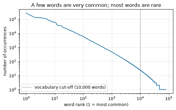
occurrences of the 10,000th most common word: 24
words that occur exactly once: 32674
The curve falls steadily: a handful of words occur hundreds of thousands of times, while the 10,000th most common word occurs only 24 times, and 32,674 words, about 40% of all distinct words, occur exactly once. This pattern, where a word's frequency falls roughly in proportion to its rank, is called Zipf's law, and it holds for almost every language and every large body of text.
It also tells us how to build a sensible vocabulary. Words that appear only once or twice are too rare for a model to learn anything reliable about. So we keep the 10,000 most common words and add two special tokens:
<pad>(ID 0): a filler token used to make short texts as long as long ones (Section 9.1).<unk>(ID 1): "unknown", used for every word that is not in the vocabulary.
We then build two lookup tables: itos ("integer to string") maps an ID to its word, and stoi ("string to integer") maps a word to its ID.
VOCAB_SIZE = 10000itos = ["<pad>", "<unk>"] + [w for w, _ in counts.most_common(VOCAB_SIZE)] # id -> wordstoi = {w: i for i, w in enumerate(itos)} # word -> idPAD, UNK = 0, 1def encode(tokens): """Map tokens through the training vocabulary, using the unknown-token policy defined above. Arguments: tokens: Ordered token strings to encode. """ return [stoi.get(w, UNK) for w in tokens]print("vocabulary size including <pad> and <unk>:", len(itos))print(tokenize(sentence))print(encode(tokenize(sentence)))print("id 2 is", repr(itos[2]), "| id", stoi["great"], "is 'great'")unk_rate = np.mean([i == UNK for doc in val_tokens for i in encode(doc)])print(f"share of validation tokens that become <unk>: {unk_rate:.1%}")vocabulary size including <pad> and <unk>: 10002 ['this', 'movie', "wasn't", 'good', 'it', 'was', 'great'] [11, 17, 291, 49, 9, 13, 80] id 2 is 'the' | id 80 is 'great' share of validation tokens that become <unk>: 6.0%
Our example sentence has become the list of numbers [11, 17, 291, 49, 9, 13, 80]. Common words get small IDs because we numbered the vocabulary by frequency: the is ID 2 (right after the two special tokens), and great is ID 80.
On the validation reviews, 6.0% of tokens are not in the vocabulary and become <unk>. That is the price of a fixed vocabulary: the model will see <unk> in place of rare names, misspellings and unusual words.
Key terms
- Token: one unit of text the model works with; here, a word.
- Tokenisation: splitting text into tokens.
- Vocabulary: the fixed list of tokens the model knows, each with a number.
- Token ID: the number of a token in the vocabulary.
<unk>/<pad>: special tokens for unknown words and for padding.
Token IDs solve the "symbols are not numbers" problem, but only on the surface. An ID is just a label, like a seat number. Word 80 is not "bigger" than word 49 in any meaningful way, and words 49 and 50 are not similar just because their numbers are close. Feeding the raw IDs into a network as if they were measurements would make it treat these arbitrary labels as quantities. We need a better way to give the network each word.
-
Our vocabulary covers 94.3% of training tokens. Why is the share of
<unk>tokens on the validation reviews (6.0%) slightly higher than the 5.7% you might expect from that figure?The vocabulary was chosen using the training reviews. Words that are common in training are, by construction, in the vocabulary; the validation reviews contain some words that were rare or absent in training (new names, rare words, typos), so slightly more of their tokens fall outside the vocabulary. This is a small, honest example of the gap between training data and new data.
Which reviews should define the vocabulary?
Training reviews, with an explicit policy for unseen validation tokens.
One-Hot Encoding and Its Limitations
The classic way to give a network a categorical value without implying any order is one-hot encoding, which you have probably used for categorical columns in classical machine learning. Each word becomes a vector as long as the vocabulary, filled with zeros except for a single 1 at the word's ID.
def one_hot(word): """Return the vocabulary-length indicator vector for a known word. Arguments: word: Vocabulary word, or tuple of BPE pieces in the merge helpers. """ v = torch.zeros(len(itos)) v[stoi[word]] = 1.0 return vgood, great, terrible = one_hot("good"), one_hot("great"), one_hot("terrible")print("one-hot length:", good.shape[0], "| non-zero entries:", int(good.sum()))print("good . great =", (good @ great).item())print("good . terrible =", (good @ terrible).item())doc_len = 200print(f"a {doc_len}-token review as one-hot vectors: {doc_len} x {len(itos)} = {doc_len * len(itos):,} numbers")one-hot length: 10002 | non-zero entries: 1 good . great = 0.0 good . terrible = 0.0 a 200-token review as one-hot vectors: 200 x 10002 = 2,000,400 numbers
Each one-hot vector has 10,002 entries, and exactly 1 of them is non-zero. One-hot vectors solve the ordering problem, since no word is "bigger" than another. But they create two new problems.
They are huge and wasteful. A single 200-token review becomes 200 × 10,002 = 2,000,400 numbers, almost all zeros.
They make every word equally different from every other word. A standard way to measure how similar two vectors are is their dot product: multiply matching entries and add them up. For one-hot vectors, the 1s are always in different places, so the dot product between any two different words is 0. As the output shows, "good" is exactly as similar to "great" (0.0) as it is to "terrible" (0.0). One-hot vectors carry no notion of meaning at all, so a model cannot transfer anything it learns about "great" to "excellent".
What we would like is a short vector for each word, made of ordinary numbers rather than mostly zeros, arranged so that similar words have similar vectors. That is exactly what an embedding is.
-
If we doubled the vocabulary to 20,000 words, what would happen to the length of each one-hot vector, and to the similarity between "good" and "great"?
Each one-hot vector would grow to about 20,000 entries (plus the special tokens). The similarity between "good" and "great" would still be exactly 0, as for any two different words. More words make one-hot vectors more wasteful, not more meaningful.
What is the dot product of two distinct one-hot vectors?
Zero; their nonzero entries occupy different coordinates.
Word Embeddings and Embedding Layers
An embedding layer is, at heart, a lookup table: a matrix with one row per word in the vocabulary. Row 49 holds the vector for "good", row 80 holds the vector for "great", and so on. To embed a token, you simply fetch its row. In PyTorch this is nn.Embedding(num_embeddings, embedding_dim), where num_embeddings is the vocabulary size and embedding_dim is the length of each vector.
The crucial point is that the table's entries are ordinary learnable parameters. They start random and are adjusted by backpropagation, like any other weights, so that the vectors become useful for the task.
torch.manual_seed(0)emb = nn.Embedding(num_embeddings=len(itos), embedding_dim=8)print("embedding table:", tuple(emb.weight.shape), "| parameters:", emb.weight.numel())ids = torch.tensor([stoi["good"], stoi["great"]])looked_up = emb(ids)via_one_hot = torch.stack([good, great]) @ emb.weightprint("lookup:\n", looked_up.detach())print("same as one-hot @ table?", torch.allclose(looked_up, via_one_hot))embedding table: (10002, 8) | parameters: 80016
lookup:
tensor([[ 1.4502, 4.1015, 1.1182, -1.5668, -0.6990, 0.5744, 1.2381, -0.6405],
[ 0.5408, -0.9478, 0.2021, -0.3507, 0.5450, 1.5412, 0.6002, -0.3380]])
same as one-hot @ table? True
Our table has shape (10002, 8): one row of 8 numbers for each of the 10,002 tokens, which makes 80,016 parameters. Looking up "good" and "great" returns their two rows. The numbers are random, because nothing has been trained yet.
The last line of the output reveals what an embedding layer really is. Multiplying a one-hot vector by the table picks out exactly one row, so an embedding lookup gives the same result as one-hot encoding followed by a linear layer, and PyTorch confirms the two are identical (True). The embedding layer just skips the wasteful multiplication by thousands of zeros and fetches the row directly.
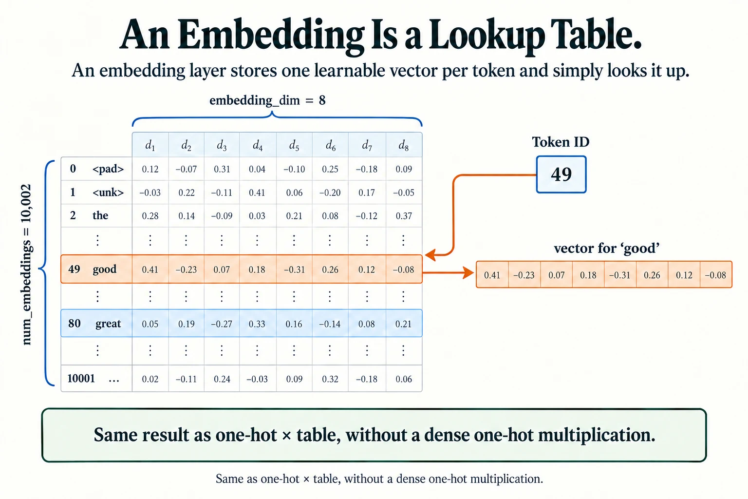
Figure 5.3.2. Selecting row 49 is equivalent to multiplying a one-hot vector by the table, without materialising that dense one-hot vector. Both table entries and the chosen row are illustrative.
Embedding layers work on whole batches of token IDs at once. A batch of shape (B, T) (B texts, each T tokens long) becomes a tensor of shape (B, T, D), adding one dimension of size D for the vector.
batch_ids = torch.tensor([encode(tokenize("the plot was great")), encode(tokenize("the acting was awful"))])print("token ids:", tuple(batch_ids.shape), "->", "embeddings:", tuple(emb(batch_ids).shape))for d in [8, 64, 300]: print(f"embedding_dim={d:>3}: {len(itos) * d:>9,} parameters")token ids: (2, 4) -> embeddings: (2, 4, 8) embedding_dim= 8: 80,016 parameters embedding_dim= 64: 640,128 parameters embedding_dim=300: 3,000,600 parameters
Two sentences of 4 tokens each, shape (2, 4), become (2, 4, 8): each of the 8 tokens has been replaced by its 8-number vector.
Common mistake: passing token IDs with a floating-point
dtypeto an embedding layer. Embedding layers need integer IDs (torch.long), because an ID is a row number, not a quantity.
Key terms
- Embedding: a learned vector of numbers that represents a token.
- Embedding layer: a learnable lookup table with one vector per vocabulary entry (
nn.Embedding).- Embedding dimension: the length of each vector (
embedding_dim).
Why does embedding lookup equal one-hot times a table?
The one nonzero entry selects the corresponding table row.
Embedding Dimensions and Vector Representations
How long should each word's vector be? The output above shows the parameter cost for our 10,002-word vocabulary: 80,016 parameters with 8 dimensions, 640,128 with 64, and 3,000,600 with 300.
It helps to think of each dimension as one "axis of meaning" that the model can use to tell words apart. With only 2 dimensions you could perhaps separate positive words from negative words, and formal words from casual ones, and nothing else. More dimensions allow more distinctions: tone, topic, grammar, whether a word is about people or objects, and so on. But nobody tells the network what each axis should mean. The axes are learned, and usually no single dimension corresponds neatly to a human concept; the meaning is spread across all of them together.
The trade-off is familiar from Module 3:
- Too few dimensions: the vectors cannot hold enough distinctions, and the model underfits.
- Too many dimensions: many more parameters to learn, which needs more data and invites overfitting, especially for rare words.
Word embeddings trained on their own typically use somewhere between tens and a few hundred dimensions; the embeddings inside large language models are much longer. In this lesson we use 32 dimensions for the sentiment model and 50 for the second model in Section 9.
-
A vocabulary has 50,000 tokens and an embedding dimension of 512. How many parameters does the embedding table have?
50,000 × 512 = 25,600,000 parameters.
Does an individual embedding coordinate have to mean one named concept?
No; useful distinctions can be distributed across coordinates.
Semantic Similarity and Cosine Similarity
If embeddings are supposed to place similar words close together, we need a way to measure "close". For word vectors, the standard measure is cosine similarity.
Imagine each vector as an arrow pointing out from the origin. Cosine similarity looks only at the angle between two arrows, not at their length:
Here a · b is the dot product from Section 4, and ‖a‖ is the length (or norm) of vector a, the square root of the sum of its squared entries. Dividing by both lengths removes the effect of size, so only direction counts. The result always lies between −1 and +1:
- +1: the arrows point in exactly the same direction.
- 0: they are at a right angle; the vectors are unrelated.
- −1: they point in exactly opposite directions.
Let's check this on small 2D vectors whose angles we can picture:
def cosine(a, b): """Return the cosine similarity of two nonzero vectors: their dot product divided by their norms. Arguments: a: First vector. b: Second vector. """ return (a @ b / (a.norm() * b.norm())).item()pairs = {"same direction": ([1., 1.], [2., 2.]), "right angle": ([1., 0.], [0., 1.]), "45 degrees": ([1., 0.], [1., 1.]), "opposite": ([1., 1.], [-1., -1.])}for name, (a, b) in pairs.items(): print(f"{name:<15} {a} vs {b}: cosine = {cosine(torch.tensor(a), torch.tensor(b)):.3f}")same direction [1.0, 1.0] vs [2.0, 2.0]: cosine = 1.000 right angle [1.0, 0.0] vs [0.0, 1.0]: cosine = 0.000 45 degrees [1.0, 0.0] vs [1.0, 1.0]: cosine = 0.707 opposite [1.0, 1.0] vs [-1.0, -1.0]: cosine = -1.000
[1, 1] and [2, 2] point the same way (one is just longer), so their cosine is 1.000, even though they are not equal. [1, 0] and [0, 1] are at a right angle: 0.000. [1, 0] and [1, 1] are 45° apart: 0.707. And [1, 1] and [−1, −1] point in opposite directions: −1.000.
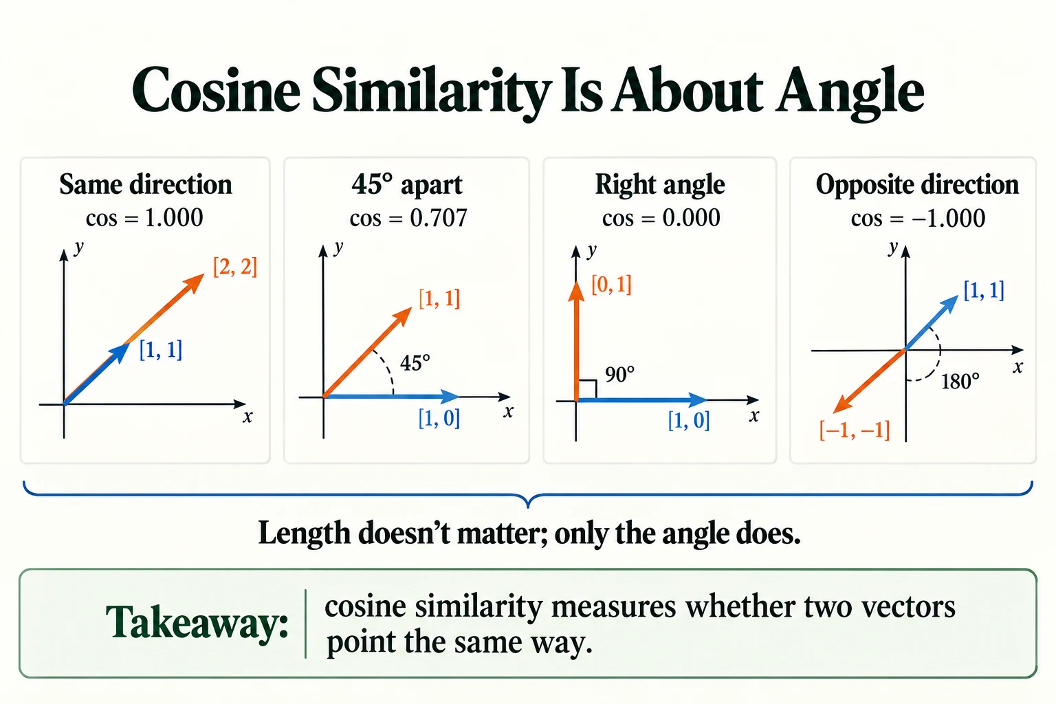
Figure 5.3.3. Cosine similarity compares directions rather than lengths: 1 for the same direction, 0 for perpendicular vectors, and −1 for opposite directions. It is undefined for a zero vector without a numerical convention.
Now apply cosine similarity to the untrained embedding table from Section 5:
def vec(table, w): """Select a known word's row from an embedding table. Arguments: table: Embedding weight matrix indexed by vocabulary ID. w: Weight tensor or selected vocabulary word, as defined in this helper. """ return table[stoi[w]]W0 = emb.weight.detach()for a, b in [("good", "great"), ("good", "terrible"), ("good", "the")]: print(f"untrained: cos({a}, {b}) = {cosine(vec(W0, a), vec(W0, b)):+.3f}")untrained: cos(good, great) = -0.081 untrained: cos(good, terrible) = -0.682 untrained: cos(good, the) = -0.714
These numbers mean nothing. "Good" comes out more similar to "great" (−0.081) than to "terrible" (−0.682) or "the" (−0.714), but that is pure luck: the table is random. With only 8 dimensions, random vectors can easily have large positive or negative cosines by chance. An embedding table becomes meaningful only after it has been trained, and, as Section 9 will show, what it becomes depends entirely on what it was trained to do.
Key terms
- Dot product: multiply matching entries of two vectors and add the results.
- Norm (length): the size of a vector, the square root of the sum of its squared entries.
- Cosine similarity: the dot product divided by both norms; it measures the angle between two vectors, from −1 to +1.
-
Two word vectors have a cosine similarity of 0.98, but one is three times as long as the other. Are they similar, according to cosine similarity?
Yes. Cosine similarity ignores length and looks only at direction. A cosine of 0.98 means the vectors point in almost the same direction, so they count as very similar, regardless of one being longer.
What does cosine similarity ignore?
Vector length; it compares directions.
Static vs. Contextual Representations
Before we train anything, there is one limitation of embedding layers that is important to understand, because it explains why the field moved on to the Transformers of Module 6.
Consider the word "bank" in these two sentences:
- She sat by the bank of the river.
- He deposited cash at the bank.
To a reader, these are two different meanings. But an embedding layer is a lookup table, and "bank" has only one row. So it must receive exactly the same vector in both sentences:
s1 = tokenize("she sat by the bank of the river")s2 = tokenize("he deposited cash at the bank")v1 = emb(torch.tensor(encode(s1)))[s1.index("bank")]v2 = emb(torch.tensor(encode(s2)))[s2.index("bank")]print("'bank' in sentence 1 vs sentence 2: cosine =", round(cosine(v1.detach(), v2.detach()), 3))'bank' in sentence 1 vs sentence 2: cosine = 1.0
The cosine similarity is 1.0: the two vectors are identical. This is called a static representation: each word gets one fixed vector, whatever its surroundings. The lookup table alone cannot change the vector of "bank" with context. A model that simply averages these vectors also loses word order and struggles with negation. An order-aware model can instead build contextual representations from the same static starting vectors.
A contextual representation, by contrast, gives each word a vector that depends on the words around it. "Bank" near "river" and "bank" near "cash" would get different vectors. Producing contextual representations requires a model that lets words exchange information with one another. Sequence models (Lesson 5.4) and, above all, Transformers (Module 6) do exactly this. They still begin with an embedding layer like ours, and then transform those static vectors into contextual ones.
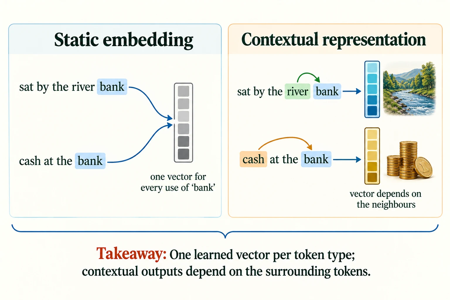
Figure 5.3.4. A static table returns the same vector for a token type in every sentence. A contextual model produces different output vectors as surrounding tokens change; a static vector can still encode multiple usages.
Key terms
- Static representation: one fixed vector per word, the same in every context.
- Contextual representation: a vector for a word that depends on the surrounding words.
-
A sentiment model averages static word embeddings to represent a review. Why might it struggle with the review "not good at all"?
The average of the static vectors for "not", "good", "at" and "all" contains the strongly positive vector for "good". Averaging cannot express that "not" reverses the meaning of "good", so the review may be scored as positive. We measured exactly this: "the movie was not good" was still scored 0.569 positive.
What distinguishes a contextual representation?
Its vector depends on surrounding tokens.
Text Embeddings in Practice with PyTorch
Now we train embeddings for real, in two different ways, and compare what they learn.
9.1 Turning reviews into a fixed-size tensor
Reviews have different lengths, but a batch must be a rectangular tensor. The standard solution has two parts:
- Truncation: cut every review to at most
MAX_LENtokens; we use 200. - Padding: fill shorter reviews up to 200 with the
<pad>token (ID 0).
MAX_LEN = 200def to_tensor(token_lists): """Truncate to MAX_LEN and pad shorter token lists with PAD; return an integer batch. Arguments: token_lists: A list of variable-length token sequences. """ X = torch.full((len(token_lists), MAX_LEN), PAD, dtype=torch.long) for i, toks in enumerate(token_lists): ids = encode(toks)[:MAX_LEN] # truncate long reviews X[i, :len(ids)] = torch.tensor(ids, dtype=torch.long) # shorter reviews stay padded return XX_train, X_val = to_tensor(train_tokens), to_tensor(val_tokens)y_train = torch.tensor((train_df.sentiment == "positive").values, dtype=torch.float32)y_val = torch.tensor((val_df.sentiment == "positive").values, dtype=torch.float32)print("X_train:", tuple(X_train.shape), "| X_val:", tuple(X_val.shape))print(f"share of training reviews longer than {MAX_LEN} tokens (truncated): {np.mean([len(t) > MAX_LEN for t in train_tokens]):.1%}")print(f"share of positions that are padding: {(X_train == PAD).float().mean().item():.1%}")X_train: (20000, 200) | X_val: (5000, 200) share of training reviews longer than 200 tokens (truncated): 40.4% share of positions that are padding: 20.9%
The training set is now a tensor of shape (20000, 200): 20,000 reviews, each exactly 200 token IDs. Truncation affects 40.4% of training reviews, which are longer than 200 tokens, and 20.9% of all positions in the tensor are padding.
Truncating that many reviews loses information, because the end of a review often contains its verdict. It is a deliberate trade-off between accuracy and speed. Padding, meanwhile, must not influence the prediction: a review should not become more negative just because it is short. We deal with that next.
9.2 Objective 1: learning embeddings for sentiment
Our first model is deliberately simple. It is a bag of embeddings: look up the vector for every token, average the vectors of the real (non-padding) tokens, and feed that one average vector to a linear layer that outputs a single score. A positive score means "positive review". The loss is BCEWithLogitsLoss, the binary cross-entropy loss for two-class problems.
The line that handles padding is the mask: it is 1 for real tokens and 0 for padding, so that padding vectors are multiplied by zero and excluded from the average. We also pass padding_idx=PAD to the embedding layer, which keeps the <pad> vector fixed at zero and never trains it.
The embedding table is trained only through the sentiment loss. The words' vectors are free to become whatever helps tell positive reviews from negative ones. We train for 4 epochs and keep the epoch with the best validation accuracy.
class BagOfEmbeddings(nn.Module): """Masked-mean word embeddings followed by a binary sentiment-logit head.""" def __init__(self, vocab_size, dim=32): """Create the components of this model; the forward computation is traced in the lesson. Arguments: vocab_size: Number of token IDs represented by the embedding table. dim: Learned vector width. """ super().__init__() self.emb = nn.Embedding(vocab_size, dim, padding_idx=PAD) self.out = nn.Linear(dim, 1) def forward(self, x): # x: (B, T) token ids """Masked-mean word embeddings followed by a binary sentiment-logit head. Arguments: x: Integer token-ID batch shaped (B, T). """ e = self.emb(x) # (B, T, D) mask = (x != PAD).unsqueeze(-1).float() # (B, T, 1): 1 for real tokens, 0 for padding mean = (e * mask).sum(1) / mask.sum(1).clamp(min=1) # (B, D): average of real tokens return self.out(mean).squeeze(-1) # (B,): one score per reviewtorch.manual_seed(0)clf = BagOfEmbeddings(len(itos))opt = torch.optim.Adam(clf.parameters(), lr=5e-3)loss_fn = nn.BCEWithLogitsLoss()snaps, val_accs = [], []for epoch in range(4): perm = torch.randperm(len(X_train)); total_loss, n = 0.0, 0 for i in range(0, len(X_train), 64): b = perm[i:i+64] opt.zero_grad(); loss = loss_fn(clf(X_train[b]), y_train[b]); loss.backward(); opt.step() total_loss += loss.item(); n += 1 with torch.no_grad(): acc = ((clf(X_val) > 0).float() == y_val).float().mean().item() val_accs.append(acc); snaps.append({k: v.clone() for k, v in clf.state_dict().items()}) print(f"epoch {epoch+1}: train loss {total_loss/n:.3f} | val acc {acc:.4f}")best = int(np.argmax(val_accs)); _ = clf.load_state_dict(snaps[best])print("best epoch on validation:", best + 1)epoch 1: train loss 0.536 | val acc 0.8272 epoch 2: train loss 0.314 | val acc 0.8578 epoch 3: train loss 0.247 | val acc 0.8646 epoch 4: train loss 0.208 | val acc 0.8632 best epoch on validation: 3
Validation accuracy rises to 0.8646 at epoch 3, then slips to 0.8632 at epoch 4 while the training loss keeps falling. That is the first sign of overfitting, so we keep the epoch 3 weights. Not bad for a model that ignores word order completely.
Now the interesting part: what did the embedding table learn? For a few words, we find the nearest neighbours: the vocabulary words whose vectors have the highest cosine similarity to that word's vector.
def neighbours(table, word, k=5): """Rank other vocabulary entries by cosine similarity to a word's embedding. Arguments: table: Embedding weight matrix indexed by vocabulary ID. word: Vocabulary word, or tuple of BPE pieces in the merge helpers. k: Number of neighbours, or unit index in unit_summary. """ T = F.normalize(table, dim=1) sims = T @ T[stoi[word]] top = sims.topk(k + 1).indices[1:] # skip the word itself return [(itos[i], round(sims[i].item(), 2)) for i in top]W_sent = clf.emb.weight.detach()for w in ["excellent", "awful", "boring", "husband", "music", "actor"]: print(f"{w:<10}", neighbours(W_sent, w))excellent [('wonderfully', 0.88), ('best', 0.85), ('fantastic', 0.85), ('snippets', 0.85), ('hilarious', 0.84)]
awful [('poorly', 0.88), ('dull', 0.88), ('waste', 0.88), ('wooden', 0.87), ('worst', 0.86)]
boring [('worst', 0.88), ('waste', 0.88), ('amateurish', 0.87), ('worse', 0.86), ('script', 0.85)]
husband [('betray', 0.61), ('aimed', 0.61), ('crude', 0.57), ('shrek', 0.56), ('mean', 0.55)]
music [('testament', 0.63), ('ida', 0.62), ('evokes', 0.62), ('uncertain', 0.57), ('aussie', 0.56)]
actor [('characterization', 0.79), ('diane', 0.72), ('superficial', 0.68), ('exercise', 0.67), ('kissing', 0.66)]
The sentiment words have very sensible neighbours. "Excellent" sits next to wonderfully, best and fantastic; "awful" sits next to poorly, dull, waste and worst. But look at the neutral words. "Husband" is next to betray, aimed and crude; "music" is next to testament, ida and evokes; "actor" is next to characterization and diane. These neighbours are less clearly related in meaning, and their similarities (around 0.55 to 0.79) are noticeably lower than those of the sentiment words (around 0.85).
This makes perfect sense once you remember what the table was trained for. The sentiment loss only ever asked one question: does this word push a review towards positive or negative? So the embeddings organised themselves along that single question. Words with no sentiment, like "husband" and "music", received no direct supervision for general semantic similarity.
9.3 Objective 2: learning embeddings from context (skip-gram)
Can we learn embeddings that capture general meaning instead? A famous idea from linguistics says yes: "You shall know a word by the company it keeps." Words that appear in similar contexts tend to have similar meanings. "Husband" and "wife" both appear near "married", "her", "his" and "divorce"; "music" and "soundtrack" both appear near "score", "songs" and "beautiful".
Skip-gram turns this idea into a training objective. It needs no labels at all, only raw text:
- Take a word in the text, the centre word.
- Look at the words up to a few positions on either side, the context words. Each (centre, context) pair is a positive example: "these two words appeared together".
- Also pick a few random words from the vocabulary, called negative samples or "noise" words. Each (centre, random word) pair is a negative example: "these probably did not appear together".
- Train two embedding tables so that the dot product of a centre word's vector with a true context word's vector is high, and with a noise word's vector is low.
This is the training method behind word2vec, one of the most influential models in natural-language processing. Because it learns from text alone, it is an example of self-supervised learning: the training labels ("did these words appear together?") come from the data itself.
First we build the training pairs. We also randomly drop many occurrences of very frequent words such as "the", a step called subsampling, because very frequent words dominate the pair counts. We build each window within one review, so the end of one review never becomes the context of another.
SG_DOCS = 15000rng = np.random.default_rng(0)docs = [np.array([i for i in encode(doc) if i > UNK], dtype=np.int64) for doc in train_tokens[:SG_DOCS]]all_ids = np.concatenate(docs)freq = np.bincount(all_ids, minlength=len(itos)) / len(all_ids)WINDOW = 5centre, context = [], []tokens_kept = 0for doc in docs: # Subsample inside each review, then form pairs inside that review only. keep = rng.random(len(doc)) < np.minimum(1.0, np.sqrt(1e-4 / np.maximum(freq[doc], 1e-12))) ids = doc[keep] tokens_kept += len(ids) for k in range(1, min(WINDOW, len(ids) - 1) + 1): centre.extend([ids[:-k], ids[k:]]) context.extend([ids[k:], ids[:-k]])centre = torch.tensor(np.concatenate(centre))context = torch.tensor(np.concatenate(context))print("reviews used:", SG_DOCS, "| window: up to", WINDOW, "words either side")print("tokens kept after subsampling:", tokens_kept, "| (centre, context) pairs:", len(centre))reviews used: 15000 | window: up to 5 words either side tokens kept after subsampling: 1307513 | (centre, context) pairs: 12625140
From 15,000 training reviews, with a window of up to 5 words on each side, subsampling keeps 1,307,513 tokens, which produce 12,625,140 (centre, context) pairs. Now we train, for one pass over all the pairs.
Inside the loop, pos is the dot-product score for each true pair and neg holds the scores for the 5 noise words of each pair. The loss uses logsigmoid, the logarithm of the sigmoid function, to push pos up and neg down. It is the same idea as binary cross-entropy, with the true pairs labelled 1 and the noise pairs labelled 0.
torch.manual_seed(0)noise = torch.tensor(np.maximum(freq, 1e-12) ** 0.75); noise /= noise.sum()E_in = nn.Embedding(len(itos), 50); E_out = nn.Embedding(len(itos), 50)nn.init.uniform_(E_in.weight, -0.01, 0.01); nn.init.zeros_(E_out.weight)opt = torch.optim.Adam(list(E_in.parameters()) + list(E_out.parameters()), lr=3e-3)perm = torch.randperm(len(centre)); B, NEG = 4096, 5print("vector size:", E_in.weight.shape[1], "| pairs per step:", B, "| random 'noise' words per pair:", NEG)losses = []for step, i in enumerate(range(0, len(centre), B)): b = perm[i:i+B]; c, o = centre[b], context[b] negs = torch.multinomial(noise, len(b) * NEG, replacement=True).view(len(b), NEG) v = E_in(c) # (B, 50) centre-word vectors pos = (v * E_out(o)).sum(-1) # (B,) score for the true context word neg = torch.bmm(E_out(negs), v.unsqueeze(-1)).squeeze(-1) # (B, NEG) scores for random words loss = -(F.logsigmoid(pos).mean() + F.logsigmoid(-neg).sum(1).mean()) opt.zero_grad(); loss.backward(); opt.step() losses.append(loss.item())print("steps:", len(losses), f"| loss first 100 steps {np.mean(losses[:100]):.3f} | last 100 steps {np.mean(losses[-100:]):.3f}")vector size: 50 | pairs per step: 4096 | random 'noise' words per pair: 5 steps: 3083 | loss first 100 steps 3.407 | last 100 steps 2.598
The loss falls from an average of 3.407 over the first 100 steps to 2.598 over the last 100. Now the same nearest-neighbour test, on the skip-gram embeddings:
W_sg = E_in.weight.detach()for w in ["excellent", "awful", "boring", "husband", "music", "actor"]: print(f"{w:<10}", neighbours(W_sg, w))excellent [('superb', 0.92), ('flawless', 0.91), ('exceptional', 0.91), ('solid', 0.91), ('ensemble', 0.9)]
awful [('terrible', 0.94), ('bad', 0.88), ('horrendous', 0.87), ('embarrassingly', 0.86), ('pathetic', 0.86)]
boring [('unnecessary', 0.92), ('lame', 0.89), ('predictable', 0.88), ('inconsistencies', 0.87), ('repetitive', 0.87)]
husband [('wife', 0.92), ('mother', 0.9), ('daughter', 0.89), ('her', 0.88), ("husband's", 0.88)]
music [('soundtrack', 0.92), ('sound', 0.87), ('songs', 0.86), ('score', 0.86), ('composed', 0.85)]
actor [('russell', 0.88), ('malcolm', 0.87), ('comedian', 0.87), ('talented', 0.87), ('clooney', 0.86)]
The neutral words now have more clearly related neighbours. "Husband" sits next to wife, mother and daughter; "music" next to soundtrack, sound, songs and score; "actor" next to comedian and talented, as well as actors' names. The sentiment words also have plausible neighbours: "excellent" next to superb, flawless and exceptional, and "awful" next to terrible, bad and horrendous. These are observations from this run, rather than guaranteed semantic groupings.
9.4 Backing the comparison with numbers
Nearest-neighbour lists are easy to cherry-pick, so let's measure the difference more systematically. We take three sets of word pairs:
- related pairs, which a reader would call similar in meaning, such as husband–wife, music–soundtrack and film–movie;
- opposite pairs with opposite sentiment, such as excellent–awful and love–hate;
- 200 random pairs drawn from the 2,000 most common words, as a baseline.
We compute the average cosine similarity within each set, for three embedding tables: a random untrained one, the sentiment one and the skip-gram one.
related = [("husband", "wife"), ("actor", "actress"), ("music", "soundtrack"), ("film", "movie"), ("funny", "hilarious"), ("boring", "dull"), ("director", "directed"), ("book", "novel")]opposite = [("excellent", "awful"), ("good", "bad"), ("best", "worst"), ("great", "terrible"), ("brilliant", "boring"), ("love", "hate")]rng = np.random.default_rng(1)random_pairs = [tuple(itos[i] for i in rng.integers(2, 2002, 2)) for _ in range(200)]rows = []torch.manual_seed(0)W_untrained = nn.Embedding(len(itos), 50).weight.detach() # random 50-dim table for comparisonfor name, table in [("untrained", W_untrained), ("sentiment", W_sent), ("skip-gram", W_sg)]: m = lambda ps: np.mean([cosine(vec(table, a), vec(table, b)) for a, b in ps]) rows.append((name, m(related), m(opposite), m(random_pairs)))print(f"{'embedding':<10} {'related':>8} {'opposite':>9} {'random':>7}")for r in rows: print(f"{r[0]:<10} {r[1]:>8.3f} {r[2]:>9.3f} {r[3]:>7.3f}")embedding related opposite random untrained -0.076 0.085 0.011 sentiment 0.141 -0.609 -0.001 skip-gram 0.830 0.495 0.408
Always read these numbers against the random column, which tells you what "no relationship" looks like in each table.
- Untrained: all three averages are close to zero (−0.076, 0.085 and 0.011). As expected, random vectors encode nothing.
- Sentiment: related pairs average only 0.141, barely above random (−0.001). But opposite pairs are strongly negative, at −0.609. This table has learned one thing very well, positive versus negative, and little else.
- Skip-gram: related pairs average 0.830, far above its random baseline of 0.408. Notice the baseline itself is high: skip-gram vectors tend to share a common overall direction, which is why comparing against random pairs matters. The surprise is the opposite pairs: 0.495, above the random baseline. To skip-gram, "excellent" and "awful" are somewhat similar, because they appear in the same kinds of contexts ("the acting was ___", "an ___ film").
Within the 20 words of the picture below, the same story shows up group by group: the family words average −0.06 under the sentiment objective and 0.87 under skip-gram, while the positive words are tightly grouped in both (0.77 and 0.83).
Here is a 2D picture of 20 words from four groups in each table. Each panel is a PCA projection (principal component analysis, a method that finds the two directions along which the points vary most and flattens everything onto them). A 2D picture of 32- or 50-dimensional vectors always loses information: these pictures keep 58% and 67% of the variation in the 20 vectors, so treat them as illustrations of the numbers above, not as proof.
from sklearn.decomposition import PCAgroups = {"positive": ["excellent", "superb", "wonderful", "great", "brilliant"], "negative": ["awful", "terrible", "boring", "worst", "dull"], "family": ["husband", "wife", "mother", "father", "sister"], "music": ["music", "soundtrack", "songs", "score", "jazz"]}colours = {"positive": "tab:green", "negative": "tab:red", "family": "tab:blue", "music": "tab:purple"}words = [w for g in groups.values() for w in g]for name, table in [("sentiment", W_sent), ("skip-gram", W_sg)]: within = {g: np.mean([cosine(vec(table, a), vec(table, b)) for i, a in enumerate(ws) for b in ws[i+1:]]) for g, ws in groups.items()} print(f"{name:<10} average cosine within each group:", " ".join(f"{g} {v:.2f}" for g, v in within.items()))fig, axes = plt.subplots(1, 2, figsize=(11, 4.6))for ax, (name, table) in zip(axes, [("sentiment embedding", W_sent), ("skip-gram embedding", W_sg)]): pca = PCA(2).fit(F.normalize(table[[stoi[w] for w in words]], dim=1).numpy()) pts = pca.transform(F.normalize(table[[stoi[w] for w in words]], dim=1).numpy()) print(f"{name}: the 2D picture keeps {pca.explained_variance_ratio_.sum():.0%} of the variation of these 20 vectors") for (x_, y_), w in zip(pts, words): g = next(k for k, v in groups.items() if w in v) ax.scatter(x_, y_, color=colours[g]); ax.annotate(w, (x_, y_), fontsize=8, xytext=(3, 3), textcoords="offset points") ax.set_title(name); ax.set_xticks([]); ax.set_yticks([])handles = [plt.Line2D([], [], marker="o", ls="", color=c, label=k) for k, c in colours.items()]fig.legend(handles=handles, loc="lower center", ncol=4); plt.tight_layout(rect=(0, 0.07, 1, 1)); plt.show()sentiment average cosine within each group: positive 0.77 negative 0.84 family -0.06 music 0.20 skip-gram average cosine within each group: positive 0.83 negative 0.71 family 0.87 music 0.82 sentiment embedding: the 2D picture keeps 58% of the variation of these 20 vectors skip-gram embedding: the 2D picture keeps 67% of the variation of these 20 vectors
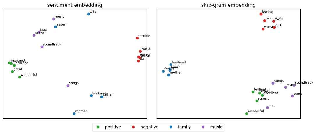
In the sentiment panel, positive and negative words form two tight clusters at opposite sides, while family and music words are scattered without structure. In the skip-gram panel, family and negative words form clear groups, while positive and music words also show structure but partly overlap in this 2D projection. The full-dimensional cosine measurements provide the stronger comparison.
This is the key lesson of this lesson: an embedding learns whatever its training objective rewards. Both demonstrations use learnable embedding tables and the same vocabulary, but they are not an objective-only controlled experiment: sentiment uses 32 dimensions and 20,000 reviews, while skip-gram uses 50 dimensions and 15,000 reviews, with a different prediction head and training procedure. The results illustrate task-shaped representations; they do not isolate the objective as the only cause of every difference. A sentiment objective builds a "sentiment axis". A context objective builds a map of how words are used, which captures topic and meaning but cannot, by itself, tell good from bad. Neither is "the true meaning" of a word; each is a representation shaped for a purpose. You saw the same idea with images in Lesson 5.1: a representation is good for a task.
9.5 The limit of static embeddings
Finally, let's go back to Section 8 and test our sentiment model on four short sentences.
tests = ["the movie was good", "the movie was not good", "the movie was bad", "the movie was not bad"]with torch.no_grad(): for t in tests: x = torch.tensor([encode(tokenize(t))]) print(f"{t:<25} P(positive) = {torch.sigmoid(clf(x)).item():.3f}")the movie was good P(positive) = 0.982 the movie was not good P(positive) = 0.569 the movie was bad P(positive) = 0.000 the movie was not bad P(positive) = 0.000
"The movie was good" gets a probability of 0.982 of being positive, and "the movie was bad" gets 0.000. So far, so good. But "the movie was not good" still gets 0.569, more likely positive than negative, and "the movie was not bad" gets 0.000, as negative as "bad" itself.
The model cannot understand negation. It sees each word's static vector, averaged together, with no idea that "not" changes the meaning of the word after it. Averaging also throws away word order completely. Fixing this needs a model that processes the words in relation to one another, which is exactly where Lesson 5.4 begins.
Common mistake: judging embeddings by a few hand-picked neighbour lists. As you saw, a sentiment table gives perfect neighbours for "awful" and nonsense for "husband". Always test several kinds of words, and compare against a random baseline.
-
According to the skip-gram embeddings, "excellent" and "awful" are more similar than two random words. Why would using those embeddings, unchanged, for sentiment analysis be risky?
Skip-gram places "excellent" and "awful" relatively close together (average opposite-pair cosine 0.495, above the random baseline of 0.408), because they appear in similar contexts. A sentiment classifier built on these vectors would start from a representation in which positive and negative words are hard to tell apart, so it would need to learn that distinction from labelled data. Embeddings from one objective are not automatically right for a different task.
What does the sentiment versus skip-gram comparison demonstrate?
Different training objectives and setups can produce different useful geometries.
Putting It All Together
Let's retrace the full path from text to meaning, now that you have built every step.
Raw text is a sequence of symbols, of varying length and inconsistent formatting, so a network cannot use it directly. Tokenisation splits it into tokens; we used lowercase words. A vocabulary of the 10,000 most frequent words covered 94.3% of training tokens, thanks to Zipf's law, with <unk> for the rest. Token IDs turn tokens into numbers, but those numbers are only labels. One-hot vectors remove the false ordering but are enormous, and make every pair of words equally different (dot product 0).
An embedding layer replaces each ID with a short, learnable vector. It is equivalent to one-hot encoding followed by a linear layer, but much cheaper. Cosine similarity measures how close two embeddings point. But the vectors mean something only after training, and they become whatever the training objective rewards:
| Embedding | Related pairs | Opposite-sentiment pairs | Random pairs |
|---|---|---|---|
| Untrained | −0.076 | 0.085 | 0.011 |
| Sentiment objective | 0.141 | −0.609 | −0.001 |
| Skip-gram objective | 0.830 | 0.495 | 0.408 |
Embedding layers are static: "bank" gets the same vector in every sentence (cosine 1.0), and a model built only from averaged static vectors cannot handle "not good" (still 0.569 positive). Getting contextual representations requires models that combine words with one another, the subject of Lesson 5.4 and Module 6.
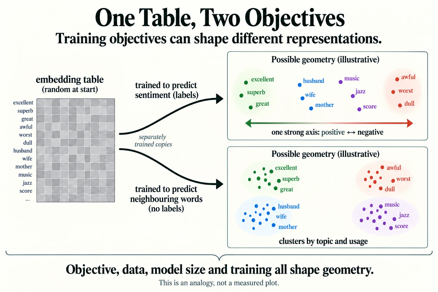
Figure 5.3.5. Illustrative geometry, not the experiment’s measured projection. Objectives, data, dimensions and training can all change an embedding space. Read the actual cosine tables and PCA plots above for evidence from this run.
Summary
- Text is a sequence of symbols of varying length; networks need fixed-size numeric tensors.
- Tokenisation splits text into tokens; every tokeniser involves choices (case, punctuation, word vs. subword).
- Word frequencies follow Zipf's law: 10,000 words covered 94.3% of training tokens, and 32,674 words appeared only once.
- Token IDs are labels, not quantities. One-hot vectors remove false ordering but are huge and express no similarity.
- An embedding layer is a learnable lookup table, equivalent to one-hot × a weight matrix. Shapes go from
(B, T)to(B, T, D). - Cosine similarity compares vectors by angle, from −1 to +1.
- Embeddings learn what their objective rewards. A sentiment objective learned a positive–negative axis (opposite pairs −0.609) but nothing about topics. Skip-gram learned topic and usage (related pairs 0.830, against a random baseline of 0.408) but puts opposite-sentiment words close together.
- Padding and truncation make text rectangular; masks keep padding out of the computation.
- Embedding layers are static; models that average them cannot handle negation or word order. Contextual models solve this.
Glossary
| Term | Meaning |
|---|---|
| Token | One unit of text the model works with (a word, subword or character). |
| Tokenisation | Splitting text into tokens. |
| Vocabulary | The fixed list of tokens a model knows, each with an ID. |
| Token ID | A token's number in the vocabulary; a label, not a quantity. |
<unk> |
Special token for words not in the vocabulary. |
<pad> |
Special filler token used to make sequences the same length. |
| Zipf's law | The pattern that a word's frequency falls roughly in proportion to its rank. |
| One-hot vector | A vector of zeros with a single 1 marking a category. |
| Embedding | A learned vector representing a token. |
| Embedding layer | A learnable lookup table of embeddings (nn.Embedding). |
| Embedding dimension | The length of each embedding vector. |
| Dot product | Sum of products of matching vector entries. |
| Norm | The length of a vector. |
| Cosine similarity | Dot product divided by both norms; measures the angle between vectors. |
| Nearest neighbours | The words whose vectors are most similar to a given word's vector. |
| Bag of embeddings | A model that averages the embeddings of a text's tokens, ignoring order. |
| Mask | A tensor of 1s and 0s marking which positions are real tokens. |
| Truncation / padding | Cutting long sequences / filling short ones to a fixed length. |
| Skip-gram | Learning embeddings by predicting which words appear near each other. |
| Negative sampling | Training against randomly chosen "noise" words that did not appear in the context. |
| Subsampling | Randomly dropping very frequent words from the training text. |
| Self-supervised learning | Learning from labels created automatically from the data itself. |
| Static representation | One fixed vector per word, regardless of context. |
| Contextual representation | A word vector that depends on the surrounding words. |
| PCA | Principal component analysis; projects data onto the directions of greatest variation. |
Wrap-up
Quick check
Which step makes token vectors learn useful task information?
Training the embedding parameters through an objective.
Why does embedding lookup equal one-hot times a table?
The one nonzero entry selects the corresponding table row.
What does the sentiment versus skip-gram comparison demonstrate?
Different training objectives and setups can produce different useful geometries.
Questions and discussion
Ask about this lesson, share what you found in a lab, or help someone else. Posts are public on the course's GitHub Discussions: anyone can read them, and you need a GitHub account to post.
Opening it loads giscus from giscus.app.