Evaluating Adapted Models
Classroom material
- Time
- ~37 min
- Sections
- 12
- Code cells
- 18
- Figures
- 4
Before you start
How do we know whether adaptation worked, and how do we decide whether to keep an adapted model?
- You will be able to
- read training curves and explain what training and validation signals tell you;
- report task metrics with confidence intervals;
- analyse errors: which reviews each method gets wrong, where methods agree, and patterns in the failures;
- identify overfitting warnings and interpret the limitations of a saved retention probe;
- compare methods on quality, trainable parameters, time and memory, with paired significance tests;
- measure run-to-run variation and track experiments;
- make and document a keep-or-reject decision by rules set in advance.
We have now adapted DistilBERT twice, fully in Lesson 8.4 and with LoRA in Lesson 8.5, and built a ladder of baselines in Lesson 8.3. Each note printed its own numbers. But a pile of numbers isn't an answer. The question that matters is: did adaptation work well enough to use? Answering it honestly takes more than reading off the highest score. We need to know whether the differences are real or noise, what kinds of mistakes each model makes, whether a model overfitted or forgot things it needed, what each method cost, and whether the results can be reproduced. Then we need a decision, made by rules we can defend, and a record of it.
This lesson does all of that, without training anything. It reads the results files saved by Lessons 8.3–8.5, checks that every method was evaluated on exactly the same reviews, and walks through a complete evaluation, ending in a keep-or-reject decision.
Key question: How do we know whether adaptation worked, and how do we decide whether to keep an adapted model?
Prerequisites
Run Lessons 8.3, 8.4 and 8.5 first to compare your own experiments. You can also study this lesson independently: it restores missing comparison files from clearly labelled author reference data, preserving any result files you already have. It uses everything from Module 8, the sign test (Module 5) and the decision record from Lesson 7.7.
Setup — imports, versions and device detection used by the notebook (1 cells)
This lesson trains no models, so it runs in seconds. The usual harmless warnings may appear, plus one "Token indices sequence length is longer than…" message in Section 4, where we count the full length of each test review on purpose.
Environment and reference results. Use Python 3.12 and requirements.txt (also supplied at the root of the Module 7/8 notebook bundle). Install packages into a separate environment, restart the kernel, and run from the beginning. The saved outputs are the author's CPU reference run, with approved explanatory corrections. Seeds and artifact revisions reduce variation; numbers and timings can differ across hardware. No account or paid API is required for the public teaching models. Initial model/data downloads require internet access.
Comparison artifacts. Missing baseline result files are restored from bundled, clearly labelled author reference data. Existing result files are preserved. Run 8.3–8.5 in the same working folder to replace these with your own experiments. The encoded reference payload in setup is delivery data; you do not need to decipher it to study the model code.
import os, json, hashlib, platformimport numpy as npimport pandas as pdimport matplotlib.pyplot as pltimport torch, transformers, peftfrom scipy.stats import binomtestfrom datasets import load_datasetfrom sklearn.feature_extraction.text import TfidfVectorizerfrom sklearn.linear_model import LogisticRegressionfrom transformers import AutoTokenizernp.random.seed(0)print("PyTorch", torch.__version__, "| Transformers", transformers.__version__, "| PEFT", peft.__version__)# Freeze the public artifacts used by the recorded experiments.MODEL_REVISIONS = {'openai/clip-vit-base-patch32': '3d74acf9a28c67741b2f4f2ea7635f0aaf6f0268', 'distilbert/distilbert-base-uncased-finetuned-sst-2-english': '714eb0fa89d2f80546fda750413ed43d93601a13', 'sentence-transformers/all-MiniLM-L6-v2': '1110a243fdf4706b3f48f1d95db1a4f5529b4d41', 'HuggingFaceTB/SmolLM2-135M': '93efa2f097d58c2a74874c7e644dbc9b0cee75a2', 'distilbert/distilgpt2': '2290a62682d06624634c1f46a6ad5be0f47f38aa', 'HuggingFaceTB/SmolLM2-135M-Instruct': '12fd25f77366fa6b3b4b768ec3050bf629380bac', 'HuggingFaceTB/SmolLM2-360M-Instruct': 'a10cc1512eabd3dde888204e902eca88bddb4951', 'Qwen/Qwen2.5-0.5B': '060db6499f32faf8b98477b0a26969ef7d8b9987', 'Qwen/Qwen2.5-7B': 'd149729398750b98c0af14eb82c78cfe92750796', 'google-bert/bert-large-uncased': '6da4b6a26a1877e173fca3225479512db81a5e5b', 'distilbert/distilbert-base-uncased': '12040accade4e8a0f71eabdb258fecc2e7e948be', 'google-bert/bert-base-uncased': '86b5e0934494bd15c9632b12f734a8a67f723594', 'cardiffnlp/twitter-roberta-base-sentiment-latest': '3216a57f2a0d9c45a2e6c20157c20c49fb4bf9c7', 'distilbert/distilbert-base-cased-distilled-squad': '564e9b582944a57a3e586bbb98fd6f0a4118db7f', 'google/vit-base-patch16-224': '3f49326eb077187dfe1c2a2bb15fbd74e6ab91e3', 'sshleifer/distilbart-cnn-12-6': 'a4f8f3ea906ed274767e9906dbaede7531d660ff', 'textattack/distilbert-base-uncased-imdb': '5b0f46c2fc4b86bf21f0ec0409bed77ee142b332', 'google/gemma-2-2b': 'c5ebcd40d208330abc697524c919956e692655cf', 'meta-llama/Llama-3.2-1B': '4e20de362430cd3b72f300e6b0f18e50e7166e08'}DATASET_REVISIONS = {'stanfordnlp/imdb': 'e6281661ce1c48d982bc483cf8a173c1bbeb5d31', 'stanfordnlp/sst2': '8d51e7e4887a4caaa95b3fbebbf53c0490b58bbb'}def benchmark_clock(): """Read elapsed time after synchronising any queued CUDA work.""" if torch.cuda.is_available(): torch.cuda.synchronize() import time return time.perf_counter()def ordered_fingerprint(texts, labels): """Hash ordered text/label pairs to verify alignment for paired comparisons. Arguments: texts: Text strings in the order expected by the caller. labels: Integer targets aligned with the input examples. """ import json, hashlib rows = [[str(t), int(y)] for t, y in zip(texts, labels)] return hashlib.sha256(json.dumps(rows, ensure_ascii=False, separators=(',', ':')).encode()).hexdigest()# Author reference results are embedded for standalone downloads, never fetched secretly.REFERENCE_RESULTS_GZIP = 'H4sIAAAAAAAC/+1bbW/bOBL+K4I/7aGJb4YvEpVFP9zt3gIH3KfdfisKQ3HkxFe/nay01y3y35ccWY4tzVByWizugEBoStMUhxy+Pc8z9NeJm+rJzdfJZluXkxv6dDXZ71bLerZYbu7LalctN/U+FKmrYrnxZRa3ukCl8kVu0Rf+VKxmpf/jv8lzbRaLsijmefimLvd1+9Vini+K3GWAt/PJ01VT2Wz/eLsvzyz5otktzAsLiP4/X0v1uLkn++vi39tqWX9J5qtiTzlU9ddJMZ8/VsX8y+QGphasf6WcF6vVbFPeT25wCseM3XYfyviMBR4/PDUN7VZk3AsqWhW35Wo/e9yXd/4FADg4YVeFjPdw9fq8Pq/P6/P6vD6vz//588Gf+O9+uf7nz79cJXjlT/ukOf8FaOLS9BxRhKxcd0GFS1V6iitcaoyAUZxyvRoVpL0atT2rUGv91Acm6J/nv3D4i8fu4tm/0++w9/k09/R7PMkF5juprn47ztuJZ/bgzEbfIpy0DJgeYbT/wNTX9wP2bPTbyPen7yupRLcf3fqwNxLQGzXs+aTbUzwb+W5/oOP1buu7b0vzB5hec77nesD5i289Z/XcT9K4oOiXvmf6be36BNgV0e251FKM+DG2hrm1B2x7QBwBfsy4OcrtGtBbX9yaA2YvQGY8JJ8AM6tRGAlpD4uNH7C7GfbWGbL1Itu6WJ8hMkuwt44hMsIojl9330R2lqHQcxDHE3rrq7t/SiXk8eH2tf6ezZ8A8g6OvXHn5y6IZwdGdyZux4Veb1E4Lbn1CMyu0gATXokIkkt5N9sVVbEu67LyaEDlmbWtGlMv10EDgikm+6AClXW93HhUMfnprZ6cYB0PLeJIJ1fYxSU5OtfFJbnS6hSY5AokpJOj7teY95BODqk7qxGNi0IdHDH4KBw5MHiYSFMYWSgEkW2/v7ik5ctPTm4j45YNN6kvhTr9XGSnqryRwsDWw/kcxS34EqgjbSFxqAMRqCOBrjg84noAEajT3+T4g56HOhJ4GII6IGyjKGxeyMy3GNTBAfgk9xqFLZ7floehTt8ODkIe6K0i+aDkoT4yM0CiJMAABGAPFhDBAog943cynhZx+wa/M/EwHQUg/GdAHc6nQ1CHm4089QKWjnxvqMP5ZSzUgcjuhSKNRYHGx85PZCE9smfNBVBHKQOGxzo6z43FDtgxU9MDOwgB7fz227trlay3d+XqKtkuFkn9UCb7h3K1kPQd11djXI49Ncal+Zkc4z9L+k7WQz3O2qxfY1CRTmrMnBJQDzJ4ASPCiizwxIAvd/pAZOUCczJx5BQYcQAjAg8OCjw8eZQRkrwTYYTMS6gHWNHi21GPJPCAiA6BlQxQpKHIID9kdgsJ9ch2gB0PEBEzslIDsLMGIoIcChiZf1Oi+cDOY36+yeIiPx9hJJGUcJ8sxvIoZmh34BAgRmUsEEaclznkUZJ2Cp5hyagHhVrGoB4U9xh+nkFULkJBlJIYFgj4HFmkEcuNISaJ5UIU48joW94VYQS6x6gMP7QrAHtKgMA6L0E9GEE9GEE98ALUc/imi3oEdcdnLzeLsio384B1co911vtkV1ZJVX5alp/PcM9DWdy9qYulRzuoXFJvP5abfQBCi2r7e7lJfl7u6+Xq7//49V3yJllt78PHua/ovir3++V2I6Ei24cwuelBGEJtJxDGZFoCRTrr1ahtH2Zp585rRB0BRWN1wKGolzRRMRIRkyczCouHF26Go17wQikIBqEhd1zDiCgQRhca3zsplvYyUCQt6TGgSI56ST6X35MjR5LUKEUtZKguCSz8cSNLnyi2SxpHFCK4MCCa8aAILwRFIESLZdkW2LWArAAjxQ1R8DwvcsryniSkShFHHC0FISsY8IQIBC8jS134PQYEMQujImtcNpYBQFwKkmCYdC+Ap4WxGCxGaINMOoelIBgFisaDMmBl/XGgSBovGA2KeFLPg04OTj1fxxkd9cqCAnMmA+VT3ZGB1mWxSXbb7cp/vEqO4Chgo6vkp7c4eXrycMJNzdntaePr8FYetnfhzvPjapUsvPXr+nHjq0l+mD/u6+3ao6ft7iqZP2z3HlfNH8r5x912uan/8r929frgjeb2dRDCfJE7goG3ZVX/9Tl5fVvsy+vHzbwInvcuKP47W5Wb+/rBD0O4pFRX4cuaYOIz0vQly912/uANePx2W9Tzh9l++bt3JaZ+MMuiCm6bVUXwri2vw93uz0W1ftwFROdfua+Ku9l8tdwdrmc3Lp3t69LnUOhPmhHF7ao8mxNpmlvfc+hMjLSJhVJeaMu6XG+rLzPv3uXaN2u2vg3VZnjF3/gSMazpYdjMqC6GzfIUz29uYTqAYWHw5haINzGk8y4ubfOoAAYCK8jugWNvbsmSfQzDysiPP9HidBgjGBbFu0cY3T0hIjnIGBa+SdiDEcKeHLoZDkpCNFw+RtiD6M0tKYgu38+6TNiTAqRjwpmS90EU4HBAQOX4DoiCJwprGgcwLM9E+ZCkdO+HQ1Ag3CwEAVePDWditMVjhD1gg5GyvAUjBDm+PpkFSYG7MeFMaQ7GhL3xGHYo8AuDtzDHhDO58ZTD8t8Dw4IgnGJEXAbxru2QsCfpRyf5HsMuttV9g7tmn7fV3ez+Mehr/tNq2/zqzZ/8B1A7udFT7QJEOIDMkGWmkB1RXnhn5nHHJ49l3r/3Jqapy9yHq/cqJHPMfVL7pAeHIWmaAiFpKVeHZEplHfpkFpJZbnzSNWV9Kg9FkTI9fgpllQppMpdmlCZ7BigdDKaodUiTxUyHujGYtGmoEcmk0jakg82MKieTGYb2YzBqNaShL8GopVYrshkKK7LoUV1Ia6qZXlTBonUQzCiyiFRHsGicCRZVsGiNCg1Ujoo7SgebxsPv4DSy6bLQcB2MWpWFd7WiMobKBLMGyawOZpX3eEiTWd2USakeTWWCXY0YnKSDXZM1ZaivmIcmm2BX62a0yG5G7TTBrs7JY4a6m1PSUDUuVG+CWZWTgw11l6yajFpGPTeOaqckGc2zULkNRo0NbbfBps6o35Zsogr+s42LgfKpr1mwY4NNA5aKBJvaAM2ujPJd6Kolo5ml/GA1BbKa0lzKHE3BYFaZUE2qqBv0akpWtU4/fGjY0DOZ2tOEp24+D4wzbSddatv3w6B/aIlidZCxZ+dx+O6tAedZQcP/7Bn/s6f871/bX/+W/FC9deHK5O6heOubk/xn5hll8ib5FP7/kYhlcljOr/wvxv9gCoAD/K8qNh8nN94e+bup5hs4YaZz69Lu2NthRqicr3NffCrvqD+Up0MD2WsjF5BE5fLBQId2buTtj/GBDhCv9F9CEkH8yUr85z0vC3QM3/64hCRKoiYvjwNLKWW4FCOJKN6FgAsDHTLwGU8SIXI/Uwp0jCOJ8UDHUJwZIwEXKcjH0y58AUlE8Wb2pSQx9pOQS0kiivMSo97DC25/SHRsmCTKgdI4SeTvYEl37+VAx8vvvMZ+iATC7JWEE/n2h7zXSD+did/+wBG3P/BCkjhWuhkX6Ijf/sBRP8IcG+j4Xrc/QLhRDheu5LhE1A10vIQkEhxdl/7FuySgST01KcaYYq5OmKI7MkUC5wemaI9MEXXLFF1+ZIqWgH9D28wzVXT2SBUtsRdsmAxmLVX0BA1bqmgPPLAhbsa0VNE4InqE8S0QIyGu6IketmzRpFq1bNHY/MgWjbWqpYs6ta4ljJZMEV/ELFUtXzQNuSQClRnd8kXlQXfLF32RrOWLJlXmmS+iafmizpo0eVcfWYlWRKGILvrqj3QRjcpauuj5EbZ0MTNWt3RRGaLoRBc9icOWLqZAg9fQRSSaTnTR9zVv6SI66qFpSJB+5otIrNkc7B75okZyMhFGnbqWSqksxSNhtDRRGsLYMF9ijMbhM2Mk2kmE0eRgjoSx4Z0NY2ySacOlXUsYtWlIJfkYSZAgwmgVdaQhjLZhiUQYieWnDTU+IYzGRgkjDXbDF+2RFZMLG77oX356+gOJoYQCOkkAAA=='def ensure_comparison_results(notes): """Restore missing author reference artifacts while preserving existing learner-generated results. Arguments: notes: Lesson IDs whose result files are required. """ import base64, gzip, json, pathlib, hashlib reference = json.loads(gzip.decompress(base64.b64decode(REFERENCE_RESULTS_GZIP))) folder = pathlib.Path('results'); folder.mkdir(exist_ok=True) for note in notes: target = folder / (note + '.json') if not target.exists(): target.write_text(json.dumps(reference[note], indent=1)) print('Using bundled AUTHOR REFERENCE results for', note, '(not a new training run).')/Users/solomonpromise/Documents/Simplilearn Classes/Deep Learning/_work78/.venv/lib/python3.12/site-packages/tqdm/auto.py:21: TqdmWarning: IProgress not found. Please update jupyter and ipywidgets. See https://ipywidgets.readthedocs.io/en/stable/user_install.html from .autonotebook import tqdm as notebook_tqdm W1017 23:21:19.379000 4811 site-packages/torch/distributed/elastic/multiprocessing/redirects.py:35] NOTE: Redirects are currently not supported in MacOs. W1017 23:21:19.471000 4811 site-packages/torch/utils/_pytree.py:630] <enum 'KernelPreference'> is an Enum subclass and is now natively supported by torch.compile as an opaque value type. Calling register_constant() on Enum subclasses is deprecated and will be an error in a future release. W1017 23:21:19.490000 4811 site-packages/torch/utils/_pytree.py:630] <enum 'ScaleCalculationMode'> is an Enum subclass and is now natively supported by torch.compile as an opaque value type. Calling register_constant() on Enum subclasses is deprecated and will be an error in a future release.
PyTorch 2.14.1 | Transformers 5.20.1 | PEFT 0.21.2
The Big Picture: How Do We Know Adaptation Worked?
"Worked" has several meanings, and a good evaluation checks each one:
| Question | Where it's answered |
|---|---|
| Did training behave sensibly? | training and validation curves (Section 2) |
| How good is the model, with what uncertainty? | task metrics with confidence intervals (Section 3) |
| What does it get wrong, and why? | error analysis (Section 4) |
| Did it overfit, or forget? | validation–test gaps, forgetting measure (Section 5) |
| Is it better than the alternatives, and at what cost? | the full comparison with paired tests (Section 6) |
| Would we get the same result again? | variation and tracking (Section 7) |
| Should we use it? | rules decided in advance (Section 8), then a written record (Section 9) |
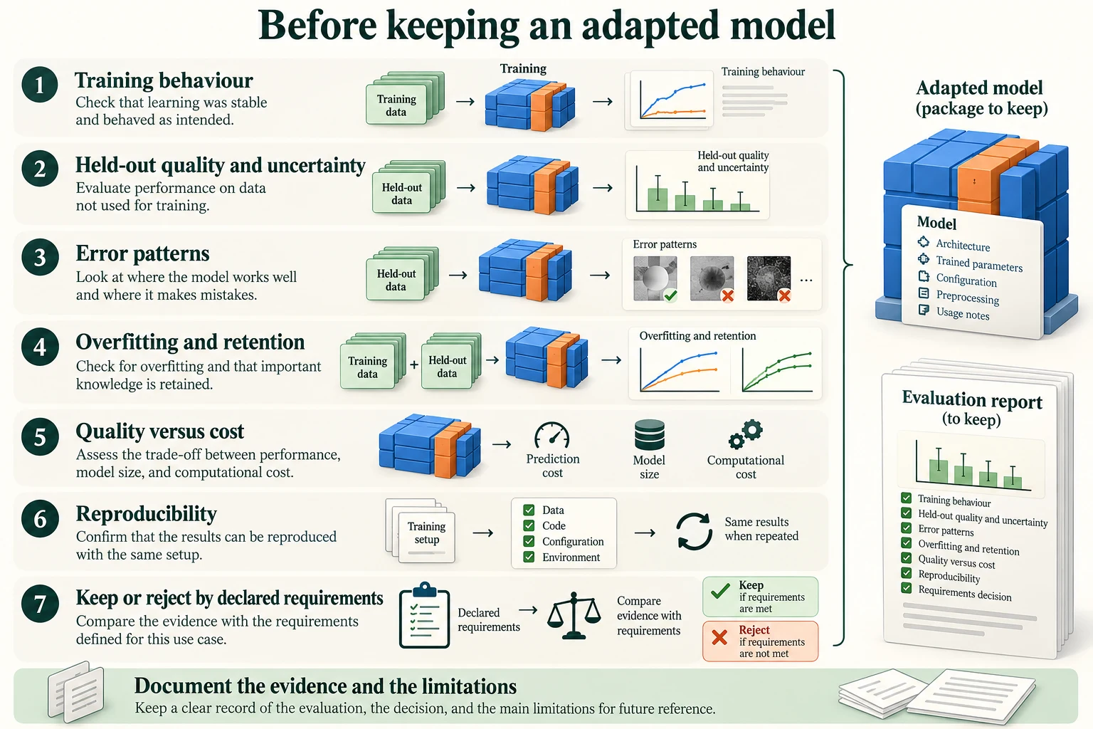
Figure 8.7.1. Evaluation combines training behaviour, held-out metrics, errors, retention, costs, reproducibility and the application decision. A p-value alone does not settle suitability.
Loading the results
The fixed split is rebuilt with the same function as every other note. Then we load the three results files and check that each one used the same split and the same 1,000 training reviews. If not, comparing them would be meaningless, so the cell stops.
def load_imdb_split(seed=0, n_val=2500, n_eval=1000, verbose=True): """Load the declared IMDb revision, remove exact duplicates and construct the seeded course splits. Arguments: seed: Seed controlling the local split or sampling generator. n_val: Number of training-half reviews reserved for validation. n_eval: Size of the reproducible evaluation subset. verbose: Whether to print dataset audit counts. """ ds = load_dataset("stanfordnlp/imdb", cache_dir="data/imdb", data_files={"train": "plain_text/train-*.parquet", "test": "plain_text/test-*.parquet"}, revision=DATASET_REVISIONS.get("stanfordnlp/imdb")) def dedup(texts, labels, seen): """Keep the first occurrence of each exact text not already in the supplied seen set. Arguments: texts: Text strings in the order expected by the caller. labels: Integer targets aligned with the input examples. seen: Set of exact texts already retained. """ keep = [] for i, t in enumerate(texts): if t not in seen: # keep only the first copy of each review seen.add(t); keep.append(i) return [texts[i] for i in keep], np.array([labels[i] for i in keep]) tr_x, tr_y = dedup(list(ds["train"]["text"]), list(ds["train"]["label"]), set()) te_x, te_y = dedup(list(ds["test"]["text"]), list(ds["test"]["label"]), set(tr_x)) # also drops test reviews already in train if verbose: print(f"official split: {len(ds['train'])} train, {len(ds['test'])} test reviews") print(f"duplicates removed: {len(ds['train']) - len(tr_x)} from train, " f"{len(ds['test']) - len(te_x)} from test (repeats, or reviews that are also in train)") clean = lambda xs: [x.replace("<br />", " ") for x in xs] # remove HTML line breaks rng = np.random.default_rng(seed) p = rng.permutation(len(tr_x)); v, t = p[:n_val], p[n_val:] # validation is carved from train q = rng.permutation(len(te_x))[:n_eval] # a fixed sample of the test set split = {"train": (clean([tr_x[i] for i in t]), tr_y[t]), "val": (clean([tr_x[i] for i in v]), tr_y[v]), "test": (clean(te_x), te_y)} split["val_eval"] = (split["val"][0][:n_eval], split["val"][1][:n_eval]) split["test_eval"] = (clean([te_x[i] for i in q]), te_y[q]) return splitdef fingerprint(texts): """Hash sorted texts to identify membership; this does not check row order or labels. Arguments: texts: Text strings in the order expected by the caller. """ return hashlib.sha256("\n".join(sorted(texts)).encode()).hexdigest()[:12]imdb = load_imdb_split()for name, (x, y) in imdb.items(): print(f"{name:<9} {len(x):>6} reviews | positive share {y.mean():.3f} | fingerprint {fingerprint(x)}")test_x, test_y = imdb["test_eval"]train_x = imdb["train"][0][:1000]Warning: You are sending unauthenticated requests to the HF Hub. Please set a HF_TOKEN to enable higher rate limits and faster downloads.
official split: 25000 train, 25000 test reviews
duplicates removed: 96 from train, 322 from test (repeats, or reviews that are also in train)
train      22404 reviews | positive share 0.502 | fingerprint fb3a1229f951
val         2500 reviews | positive share 0.492 | fingerprint 07758bc36c9b
test       24678 reviews | positive share 0.503 | fingerprint 429c5557b6d4
val_eval    1000 reviews | positive share 0.495 | fingerprint 9934ffeaac91
test_eval   1000 reviews | positive share 0.515 | fingerprint fc9fa98701bc
ensure_comparison_results(["8.3", "8.4", "8.5"])need = {"8.3": "results/8.3.json", "8.4": "results/8.4.json", "8.5": "results/8.5.json"}missing = [n for n, f in need.items() if not os.path.exists(f)]assert not missing, f"run Note(s) {', '.join(missing)} first: their results files are missing"files = {n: json.load(open(f)) for n, f in need.items()}expected = {k: fingerprint(imdb[k][0]) for k in ("train", "val_eval", "test_eval")}for n, rec in files.items(): ok = rec["split_fingerprints"] == expected and rec["train_subset_fingerprint"] == fingerprint(train_x) print(f"Note {n}: same split and same 1,000 training reviews: {ok}") assert ok, f"Note {n} was run on different data: rerun it"# The legacy membership digest does not establish prediction order. New runs# also record the ordered text/label digest; bundled original records are# explicitly identified as source reference artifacts, with their declared order.for note, rec in files.items(): ordered = rec.get('ordered_test_fingerprint') if ordered is not None: assert ordered == ordered_fingerprint(test_x, test_y), 'Prediction ordering differs: ' + noteNote 8.3: same split and same 1,000 training reviews: True Note 8.4: same split and same 1,000 training reviews: True Note 8.5: same split and same 1,000 training reviews: True
All three notes ran on the same data. Here is everything they measured, side by side:
methods = {}for name, r in files["8.3"]["rungs"].items(): methods[name] = rmethods["full fine-tuning"] = files["8.4"]methods["LoRA"] = files["8.5"]for name, r in methods.items(): print(f"{name:<40} labels {r['labels_used']:>6,} | val {r['val']['accuracy']:.3f} | test {r['test']['accuracy']:.3f}")majority class labels 1,000 | val 0.505 | test 0.485 TF-IDF, 1,000 labels labels 1,000 | val 0.866 | test 0.828 TF-IDF, all labels labels 22,404 | val 0.921 | test 0.913 SST-2 model, off the shelf labels 0 | val 0.888 | test 0.873 frozen DistilBERT + logistic regression labels 1,000 | val 0.850 | test 0.837 full fine-tuning labels 1,000 | val 0.860 | test 0.834 LoRA labels 1,000 | val 0.880 | test 0.834
Seven methods, all scored on the same 1,000 validation and 1,000 test reviews. The rest of this lesson works out what these numbers mean.
What must be checked before combining result files?
Their provenance and aligned evaluation identities.
Training vs. Validation Loss
During training, two kinds of signal tell you whether things are going well. The training loss shows whether the model is fitting the data it learns from. A validation signal, validation loss or validation accuracy on data the model never trains on, shows whether that learning carries over to new data. Overfitting appears as the two pulling apart: training keeps improving while validation stalls or worsens (Lesson 8.1).
Lessons 8.4 and 8.5 saved the training loss at every step and the validation accuracy at each checkpoint:
fig, axes = plt.subplots(1, 2, figsize=(10, 3.6))for name, colour in (("full fine-tuning", "tab:orange"), ("LoRA", "tab:blue")): s, l = zip(*methods[name]["train_loss_curve"]) smooth = np.convolve(l, np.ones(8) / 8, mode="valid") axes[0].plot(s[7:], smooth, color=colour, label=name) cs, ca = zip(*methods[name]["val_checkpoints"]) axes[1].plot(cs, ca, "o-", color=colour, label=name)axes[0].set_title("training loss (average of 8 steps)"); axes[0].set_xlabel("step")axes[1].set_title("validation accuracy (200 reviews)"); axes[1].set_xlabel("step")for a in axes: a.grid(alpha=0.3); a.legend()plt.tight_layout(); plt.show()for name in ("full fine-tuning", "LoRA"): l = [v for _, v in methods[name]["train_loss_curve"]] print(f"{name:<17} training loss: first 8 steps {np.mean(l[:8]):.3f} -> last 8 steps {np.mean(l[-8:]):.3f} | " f"chosen step {methods[name]['settings']['chosen_step']} | validation (1,000) {methods[name]['val']['accuracy']:.3f}")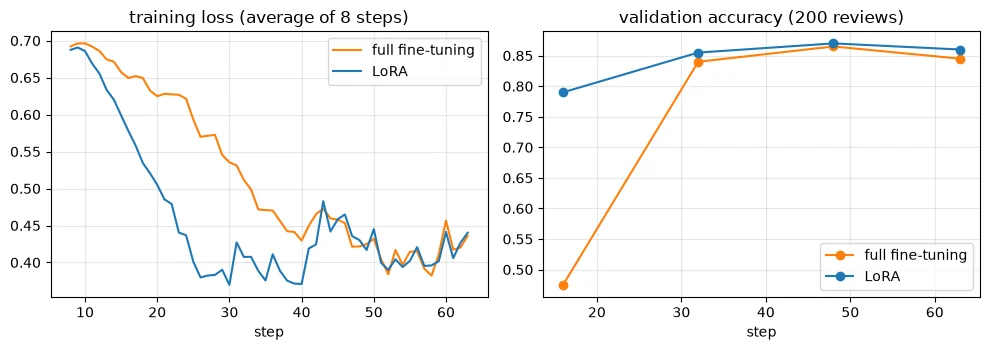
full fine-tuning  training loss: first 8 steps 0.692 -> last 8 steps 0.436 | chosen step 48 | validation (1,000) 0.860
LoRA              training loss: first 8 steps 0.688 -> last 8 steps 0.440 | chosen step 48 | validation (1,000) 0.880
Both runs started at a training loss near ln 2 (0.692 and 0.688 over the first 8 steps, the untrained-head value from Lesson 8.4) and ended at 0.436 and 0.440 over the last 8 steps. LoRA's loss fell faster early on, mostly because of its larger learning rate, and its first checkpoint was already far above chance, while full fine-tuning's was still at chance. Both peaked on validation at step 48 and dipped slightly at the end: a mild sign that one epoch was about right, and that checkpoint selection mattered.
A note on what we didn't record: validation loss. Validation accuracy only counts right and wrong; validation loss also shows whether the model is becoming over-confident on the reviews it gets wrong, often an earlier sign of overfitting. Recording it costs nothing extra during evaluation, and an experiment record should include it. That's a lesson for the next run, not something to invent now.
Key terms
- Training loss: the loss on the batches being trained on; shows whether the model fits its training data.
- Validation loss / accuracy: the same measures on held-out data; shows whether learning generalises.
Does a lower training loss establish a better deployed model?
No; held-out quality and application constraints still matter.
Task-Specific Metrics
Our task's metrics are accuracy, recall on each class, and F1 for the positive class (Lesson 8.2). Any accuracy measured on 1,000 reviews is uncertain, so we add a 95% confidence interval: a range that, by a standard calculation (the Wilson interval), is likely to contain the accuracy we'd see on unlimited reviews like these.
def wilson(k, n, z=1.96): """Calculate a Wilson confidence interval for a binomial proportion under the stated normal quantile. Arguments: k: Number of successful observations. n: Total number of binomial observations. z: Normal quantile used for the Wilson interval. """ p = k / n; d = 1 + z * z / n c = (p + z * z / (2 * n)) / d; h = z * np.sqrt(p * (1 - p) / n + z * z / (4 * n * n)) / d return c - h, c + hrows = []for name, r in methods.items(): pred = np.array(r["test_pred"]) k = int((pred == test_y).sum()) lo, hi = wilson(k, len(test_y)) rows.append({"method": name, "accuracy": k / len(test_y), "95% interval": f"{lo:.3f}-{hi:.3f}", "recall neg": r["test"]["recall_neg"], "recall pos": r["test"]["recall_pos"], "F1 pos": r["test"]["f1_pos"]})table = pd.DataFrame(rows).set_index("method")print(table.round(3).to_string())accuracy 95% interval recall neg recall pos F1 pos method majority class 0.485 0.454-0.516 1.000 0.000 0.000 TF-IDF, 1,000 labels 0.828 0.803-0.850 0.821 0.835 0.833 TF-IDF, all labels 0.913 0.894-0.929 0.920 0.907 0.915 SST-2 model, off the shelf 0.873 0.851-0.892 0.856 0.889 0.878 frozen DistilBERT + logistic regression 0.837 0.813-0.859 0.835 0.839 0.841 full fine-tuning 0.834 0.810-0.856 0.874 0.796 0.832 LoRA 0.834 0.810-0.856 0.829 0.839 0.839
The intervals are roughly four to five points wide. Full fine-tuning and LoRA both score 0.834, with intervals of 0.810–0.856. The off-the-shelf SST-2 model scores 0.873 (0.851–0.892), and TF-IDF with all labels 0.913 (0.894–0.929). Overlapping intervals don't settle a comparison on their own; for that we use the paired sign test (Section 6), which is more sensitive because it compares methods review by review.
The recall columns show a difference the accuracies hide. Full fine-tuning catches negative reviews well (0.874) but misses more positive ones (0.796), while LoRA is balanced (0.829 and 0.839). If the feature's purpose were to catch unhappy customers, full fine-tuning's profile might even be preferable, despite equal accuracy. Metrics should match what the application needs (Lesson 7.5).
Key terms
- Confidence interval: a range likely to contain the true value of a measured quantity; here, accuracy on unlimited data.
- Wilson interval: a standard way to compute a confidence interval for a proportion.
-
Two models' 95% intervals overlap. Does that prove there's no real difference between them? What would you do instead?
No. Overlapping 95% intervals are consistent with a real difference, because each interval reflects the uncertainty of one model on its own, ignoring that both were scored on the same reviews. A paired test, such as the sign test on the reviews where exactly one model is right, uses that pairing and can detect differences that overlapping intervals hide.
What does an accuracy confidence interval describe?
Sampling uncertainty under its stated assumptions.
Qualitative Evaluation and Error Analysis
4.1 Who gets what wrong
Metrics count errors; error analysis looks at them. First, how much do methods agree on which reviews are hard? The table counts test reviews that both the row's and the column's method got wrong. The diagonal shows each method's own number of errors.
names = ["TF-IDF, 1,000 labels", "frozen DistilBERT + logistic regression", "SST-2 model, off the shelf", "full fine-tuning", "LoRA", "TF-IDF, all labels"]short = {"TF-IDF, 1,000 labels": "TF-IDF 1k", "frozen DistilBERT + logistic regression": "frozen", "SST-2 model, off the shelf": "SST-2", "full fine-tuning": "full FT", "LoRA": "LoRA", "TF-IDF, all labels": "TF-IDF all"}wrong = {n: np.array(methods[n]["test_pred"]) != test_y for n in names}overlap = pd.DataFrame([[int((wrong[a] & wrong[b]).sum()) for b in names] for a in names], index=[short[n] for n in names], columns=[short[n] for n in names])print("test reviews both methods got wrong (diagonal: each method's own errors):")print(overlap.to_string())test reviews both methods got wrong (diagonal: each method's own errors):
TF-IDF 1k frozen SST-2 full FT LoRA TF-IDF all
TF-IDF 1k 172 74 46 67 68 68
frozen 74 163 65 85 106 47
SST-2 46 65 127 77 84 31
full FT 67 85 77 166 112 42
LoRA 68 106 84 112 166 44
TF-IDF all 68 47 31 42 44 87
Full fine-tuning and LoRA each get 166 reviews wrong, and 112 of those are shared. They're the same model architecture trained on the same data, so they fail in similar places. LoRA also shares 106 errors with the frozen encoder: all three use the same pretrained DistilBERT representation, which seems to struggle with the same reviews. The SST-2 model and TF-IDF with all labels share far fewer errors with the others: they fail differently.
4.2 Patterns
both_ft = wrong["full fine-tuning"] & wrong["LoRA"]print(f"wrong for both fine-tuned models: {both_ft.sum()} | of those, right for the SST-2 model: {(both_ft & ~wrong['SST-2 model, off the shelf']).sum()}")print(f"wrong for every one of the {len(names)} methods: {np.logical_and.reduce([wrong[n] for n in names]).sum()}")tok = AutoTokenizer.from_pretrained("distilbert/distilbert-base-uncased", revision=MODEL_REVISIONS.get("distilbert/distilbert-base-uncased"))n_tok = np.array([len(ids) for ids in tok(test_x, add_special_tokens=True)["input_ids"]])for label, mask in (("fits in 128 tokens", n_tok <= 128), ("longer than 128 tokens", n_tok > 128)): accs = " | ".join(f"{short[n]} {1 - wrong[n][mask].mean():.3f}" for n in names) print(f"{label:<23} ({mask.sum():>3} reviews): {accs}")wrong for both fine-tuned models: 112 | of those, right for the SST-2 model: 46 wrong for every one of the 6 methods: 12
[transformers] Token indices sequence length is longer than the specified maximum sequence length for this model (903 > 512). Running this sequence through the model will result in indexing errors
fits in 128 tokens      (121 reviews): TF-IDF 1k 0.818 | frozen 0.909 | SST-2 0.917 | full FT 0.884 | LoRA 0.876 | TF-IDF all 0.909
longer than 128 tokens  (879 reviews): TF-IDF 1k 0.829 | frozen 0.827 | SST-2 0.867 | full FT 0.827 | LoRA 0.828 | TF-IDF all 0.914
Of the 112 reviews both fine-tuned models got wrong, the SST-2 model got 46 right, so those are worth reading. Only 12 reviews defeat all six methods, perhaps hard or even mislabelled ones. Splitting by length shows something else. On the 121 test reviews that fit within 128 tokens, the DistilBERT-based methods all do well (0.876–0.917). On the 879 longer reviews, which head+tail truncation had to cut, every method that reads only 128 tokens drops, while TF-IDF with all labels, which reads every word, holds at 0.914. Part of the gap between the transformer methods and that TF-IDF model is simply that TF-IDF saw the whole review.
Here are the first three reviews that both fine-tuned models got wrong but the SST-2 model got right:
idx = np.where(both_ft & ~wrong["SST-2 model, off the shelf"])[0][:3] # the first three such reviewsfor i in idx: print(f"\ntrue: {'positive' if test_y[i] else 'negative'} | {n_tok[i]} tokens") print(" " + test_x[i][:280] + " ...")true: positive | 367 tokens That's a bad, raunchy, predictable, tacky, salacious soap opera? "The Best of Everything" is just such a guilty pleasure for me, something along the lines of "Valley of the Dolls". I mean, "Best" has everything. Somebody gets pregnant out of wedlock (when's the last time you hear ... true: positive | 175 tokens The main reason to check this one out is to watch Laura Gemser in all her glory. That's reason enough for me. She heads to Africa as guests of another rich guy that seems to be all over these films. Huge mansion near the jungle. Hunters staying around for parties when they aren ... true: positive | 281 tokens With all the shoot em up, blood horror movies that have come our way in the last little while "Saw, Hostal, Saw 2, The Hills have eyes" Yes, they have their place, don't get me wrong! I went to see "When a stranger calls" with my buddy the other night! Why? Because it's a remake ...
All three are positive reviews written with plenty of negative-sounding words. One calls the film "a bad, raunchy, predictable, tacky, salacious soap opera" and then a "guilty pleasure". One praises the film for a reason other than its quality. One opens by comparing it with gory horror films. The fine-tuned models, trained on just 1,000 reviews, seem to have learned that negative words mean a negative review. The SST-2 model, trained on many more labelled sentences, handles the reversal. That points to a concrete improvement: more training examples of exactly this kind of review.
Key terms
- Error analysis: examining which examples a model gets wrong, and why.
- Error overlap: how many errors two models share; low overlap means they fail differently, which also makes them good candidates to combine.
Common mistake: choosing error examples by hand because they "look interesting". Choose them by a rule (here, the first three that meet a condition), or you may be picking the examples that support a story you already believe.
Why inspect error overlap?
Equal aggregate accuracy can hide different individual failures.
Detecting Overfitting and Catastrophic Forgetting
5.1 The validation–test gap
Settings (regularisation, checkpoints) were chosen on validation, so each method's validation score is slightly optimistic, and the test score is the honest one. A large gap between them warns that a method was tuned to its validation data, a form of overfitting to the selection process.
for name in ("TF-IDF, 1,000 labels", "frozen DistilBERT + logistic regression", "full fine-tuning", "LoRA"): r = methods[name] print(f"{name:<40} validation {r['val']['accuracy']:.3f} | test {r['test']['accuracy']:.3f} | gap {r['val']['accuracy'] - r['test']['accuracy']:+.3f}")TF-IDF, 1,000 labels validation 0.866 | test 0.828 | gap +0.038 frozen DistilBERT + logistic regression validation 0.850 | test 0.837 | gap +0.013 full fine-tuning validation 0.860 | test 0.834 | gap +0.026 LoRA validation 0.880 | test 0.834 | gap +0.046
All four methods that chose settings on validation score lower on test, by between 0.013 and 0.046. LoRA has the largest gap (0.880 → 0.834): its validation score looked best among the 1,000-label methods, but on test it is level with the rest. That is why final test reporting must remain separate from selecting settings on validation, and why a single validation result should never be trusted on its own (Section 7 shows how much results vary).
5.2 Forgetting
Interpret the evidence carefully. A validation–test gap alone cannot diagnose overfitting: sampling variation and selection on validation can also produce one. Examine training and held-out learning curves, and reserve a fresh final test after any further model selection.
f4, f5 = methods["full fine-tuning"]["forgetting_word_guessing_loss"], methods["LoRA"]["forgetting_word_guessing_loss"]print(f"word-guessing loss on 200 held-out reviews: pretrained {f4['pretrained']} | full fine-tuning {f4['fine-tuned']} | " f"LoRA merged {f5['LoRA merged in']} | LoRA switched off: unchanged by construction")word-guessing loss on 200 held-out reviews: pretrained 3.381 | full fine-tuning 4.07 | LoRA merged 3.461 | LoRA switched off: unchanged by construction
The forgetting measure from Lesson 8.1 tells a clear story: full fine-tuning raised the word-guessing loss from 3.381 to 4.07, while LoRA, even merged, raised it only to 3.461, and with the adapter switched off it is unchanged. For this application we don't need word-guessing, so forgetting doesn't count against either model here. In applications where the adapted model must keep general abilities, it would weigh heavily in LoRA's favour.
-
Why is a validation–test gap expected for every method that chose settings on validation, and when should a gap worry you?
Choosing settings or checkpoints on validation picks whichever option was luckiest there, so part of the validation score is that luck, and it doesn't carry over to test. A small drop is therefore normal. A gap should worry you when it's much larger than the run-to-run variation you'd expect (here about two points), or when it's large for one method but not others evaluated the same way. That suggests the method was tuned to quirks of the validation set, or that something leaked.
Does one retention probe measure every old capability?
No; it tests a specific setup and requires careful interpretation.
Comparing Across the Ladder: Performance, Trainable Parameters, Time, Memory
6.1 The whole ladder
Here is every method with what it used and what it cost. Training times were measured in each note on this machine and printed with units; compare them relative to each other, since they vary between machines and runs.
cost = {"majority class": (0, "-"), "TF-IDF, 1,000 labels": (methods["TF-IDF, 1,000 labels"]["trained_parameters"], methods["TF-IDF, 1,000 labels"]["train_time"]), "TF-IDF, all labels": (methods["TF-IDF, all labels"]["trained_parameters"], methods["TF-IDF, all labels"]["train_time"]), "SST-2 model, off the shelf": (0, "-"), "frozen DistilBERT + logistic regression": (methods["frozen DistilBERT + logistic regression"]["trained_parameters"], methods["frozen DistilBERT + logistic regression"]["train_time"]), "full fine-tuning": (methods["full fine-tuning"]["trainable_parameters"], methods["full fine-tuning"]["train_time"]), "LoRA": (methods["LoRA"]["trainable_parameters"], methods["LoRA"]["train_time"])}mem = {"full fine-tuning": f"{methods['full fine-tuning']['training_memory_estimate_mb']} MB", "LoRA": f"{methods['LoRA']['training_memory_estimate_mb']} MB"}comp = pd.DataFrame([{"method": n, "labels": methods[n]["labels_used"], "trained params": cost[n][0], "train time": cost[n][1], "training memory": mem.get(n, "-"), "test acc": methods[n]["test"]["accuracy"]} for n in cost]).set_index("method")print(comp.to_string())labels trained params train time training memory test acc method majority class 1000 0 - - 0.485 TF-IDF, 1,000 labels 1000 29755 0.1 s - 0.828 TF-IDF, all labels 22404 399451 4.2 s - 0.913 SST-2 model, off the shelf 0 0 - - 0.873 frozen DistilBERT + logistic regression 1000 769 9.9 s - 0.837 full fine-tuning 1000 66955010 58 s 1071 MB 0.834 LoRA 1000 739586 45 s 280 MB 0.834
The costs span orders of magnitude:
- TF-IDF trains tens or hundreds of thousands of word weights in seconds.
- The frozen encoder trains 769 weights after one feature pass.
- LoRA trains 739,586 parameters, full fine-tuning all 66,955,010. Their estimated training memory is 280 MB and 1071 MB.
- The SST-2 model trains nothing on IMDb. Note, though, that it isn't free in an absolute sense: someone else fine-tuned it on a large labelled dataset, and we inherit that work.
6.2 Is anything better than the best cheap baseline?
The strongest method using no more than 1,000 IMDb labels is the SST-2 model off the shelf. We compare everything with it on the same test reviews:
best_baseline = "SST-2 model, off the shelf" # the strongest method using <= 1,000 labelsref = np.array(methods[best_baseline]["test_pred"]) == test_yfor name in ("full fine-tuning", "LoRA", "frozen DistilBERT + logistic regression", "TF-IDF, 1,000 labels", "TF-IDF, all labels"): right = np.array(methods[name]["test_pred"]) == test_y a, b = int((right & ~ref).sum()), int((~right & ref).sum()) print(f"{name:<40} vs {best_baseline}: only it right {a:>3} | only baseline right {b:>3} | p = {(binomtest(a, a + b).pvalue if a + b else 1.0):.2g}")full fine-tuning vs SST-2 model, off the shelf: only it right 50 | only baseline right 89 | p = 0.0012 LoRA vs SST-2 model, off the shelf: only it right 43 | only baseline right 82 | p = 0.00062 frozen DistilBERT + logistic regression vs SST-2 model, off the shelf: only it right 62 | only baseline right 98 | p = 0.0055 TF-IDF, 1,000 labels vs SST-2 model, off the shelf: only it right 81 | only baseline right 126 | p = 0.0022 TF-IDF, all labels vs SST-2 model, off the shelf: only it right 96 | only baseline right 56 | p = 0.0015
Every 1,000-label method is significantly worse than the off-the-shelf model:
- full fine-tuning: 50 against 89 reviews, p = 0.0012;
- LoRA: 43 against 82, p = 0.00062;
- the frozen encoder and TF-IDF with 1,000 labels likewise.
Only TF-IDF trained on all 22,404 labels beats it (96 against 56, p = 0.0015). The picture in one chart:
fig, ax = plt.subplots(figsize=(7, 3.8))for n in cost: if n == "majority class": continue x = max(cost[n][0], 1) ax.scatter(x, methods[n]["test"]["accuracy"], s=60) ax.annotate(n.replace(", off the shelf", "\n(off the shelf)").replace(" + logistic regression", "\n+ head"), (x, methods[n]["test"]["accuracy"]), fontsize=7, xytext=(5, 4), textcoords="offset points")ax.set_xscale("log"); ax.set_xlabel("parameters trained on IMDb (log scale; 1 = none)"); ax.set_ylabel("test accuracy (1,000 reviews)")ax.set_title("What each method trained, and what it scored"); ax.grid(alpha=0.3); ax.set_ylim(0.8, 0.93); plt.show()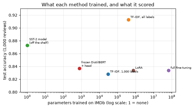
The chart makes the lesson hard to miss. Training more parameters on the same 1,000 labels didn't buy accuracy: the frozen encoder (769 parameters), LoRA (739,586) and full fine-tuning (66,955,010) all land at about the same height. The two winners got their advantage from more labelled data: the SST-2 model indirectly, through someone else's large dataset, and TF-IDF directly, from all 22,404 IMDb labels.
-
A colleague concludes "fine-tuning doesn't work for sentiment analysis". What's wrong with that conclusion, given what was and wasn't varied here?
It generalises far beyond what was tested. We fine-tuned one small model, on only 1,000 labels, for one epoch, with 128 tokens of each review and untuned learning rates, on a CPU. The comparison showed that, in this setup, fine-tuning didn't beat a model already fine-tuned on much more sentiment data, or TF-IDF with all labels. With more labels, longer inputs or a better-tuned recipe, the result could change. The correct conclusion is limited to the conditions tested, which is exactly what the decision record's limitations say.
What should a fair comparison disclose?
Data budgets, input policy, tuning budget, quality and costs.
Reproducibility and Experiment Tracking
7.1 How much do results vary?
Every adapted model here comes from a single training run. How much might a result change with a different random draw? We can't afford to retrain the Transformers many times on a CPU, but we can measure the variation for the cheapest rung: TF-IDF trained on five different random sets of 1,000 training reviews, scored on the same validation reviews.
val_x, val_y = imdb["val_eval"]all_x, all_y = imdb["train"]rng = np.random.default_rng(0)accs = []for draw in range(5): # 5 different sets of 1,000 training reviews idx = rng.choice(len(all_x), 1000, replace=False) vec = TfidfVectorizer(min_df=2, ngram_range=(1, 2), sublinear_tf=True) X = vec.fit_transform([all_x[i] for i in idx]) clf = LogisticRegression(C=3, max_iter=2000).fit(X, all_y[idx]) accs.append((clf.predict(vec.transform(val_x)) == val_y).mean())print("TF-IDF, 1,000 labels, five different training draws: validation accuracy", [round(float(a), 3) for a in accs], f"| spread {min(accs):.3f}-{max(accs):.3f}")TF-IDF, 1,000 labels, five different training draws: validation accuracy [0.846, 0.853, 0.84, 0.851, 0.859] | spread 0.840-0.859
Validation accuracy ranges from 0.840 to 0.859 across the five draws, about two points, purely from which 1,000 reviews were labelled. Fine-tuning runs also vary with initialisation, shuffling and dropout. So differences of one or two points between single runs, like LoRA's 0.880 against full fine-tuning's 0.860 on validation, shouldn't be read as real without repeated runs or a paired test. The paired test said there was no difference on test (Lesson 8.5).
7.2 Tracking experiments
Each note saved its settings, data fingerprints, costs and results to a file. Collecting them into one table, and saving it, is the beginning of experiment tracking: a permanent, comparable record of every run. Tools such as MLflow and Weights & Biases do this at scale, but the principle is the same.
tracking = pd.DataFrame([{"note": "8.3" if n in files["8.3"]["rungs"] else ("8.4" if n == "full fine-tuning" else "8.5"), "method": n, "setting": json.dumps(methods[n].get("settings", methods[n].get("setting", ""))), "val_acc": methods[n]["val"]["accuracy"], "test_acc": methods[n]["test"]["accuracy"]} for n in methods])os.makedirs("results", exist_ok=True)tracking.to_csv("results/experiments.csv", index=False)print(tracking[["note", "method", "val_acc", "test_acc"]].to_string(index=False))print("environment:", {"python": platform.python_version(), "torch": torch.__version__, "transformers": transformers.__version__, "peft": peft.__version__})note method val_acc test_acc
8.3 majority class 0.505 0.485
8.3 TF-IDF, 1,000 labels 0.866 0.828
8.3 TF-IDF, all labels 0.921 0.913
8.3 SST-2 model, off the shelf 0.888 0.873
8.3 frozen DistilBERT + logistic regression 0.850 0.837
8.4 full fine-tuning 0.860 0.834
8.5 LoRA 0.880 0.834
environment: {'python': '3.12.15', 'torch': '2.14.1', 'transformers': '5.20.1', 'peft': '0.21.2'}
The table lists every method with its note, settings, validation and test accuracy, and is saved as results/experiments.csv, alongside the environment (Python 3.12.15, PyTorch 2.14.1, Transformers 5.20.1, PEFT 0.21.2). With the fixed split, the fingerprints and the pinned versions in requirements.txt, anyone can rerun these lessons and check the numbers.
Key terms
- Run-to-run variation: differences in results caused by randomness in data sampling, initialisation and training order.
- Experiment tracking: recording each run's settings, data, code versions and results so that runs can be compared and reproduced.
What does repeated TF-IDF training on different samples measure?
Variation from those data draws, not every neural seed effect.
The Keep-or-Reject Decision
A decision should follow rules written before looking at which model looks best. Otherwise it's easy to find reasons to keep the model you hoped would win. Ours, stated in the cell below before the decision is computed:
- R1: an adapted model must beat the strongest baseline that uses no more labels, on the same test reviews, with sign-test p < 0.05.
- R2: it must fit the deployment budget (CPU inference, one model per task). All candidates do.
- R3: it must not damage abilities we still need. Word-guessing isn't needed here.
rules = { "R1": "it must beat the strongest baseline that uses no more labels, on the same test reviews, with sign-test p < 0.05", "R2": "it must fit the deployment budget: CPU inference, one model per task", "R3": "it must not damage abilities we still need (we do not need word-guessing here)",}ref = np.array(methods[best_baseline]["test_pred"]) == test_ydecision = {}for name in ("full fine-tuning", "LoRA"): right = np.array(methods[name]["test_pred"]) == test_y a, b = int((right & ~ref).sum()), int((~right & ref).sum()) p = (binomtest(a, a + b).pvalue if a + b else 1.0) r1 = a > b and p < 0.05 decision[name] = "keep" if r1 else "reject" print(f"{name:<17} R1: {'passes' if r1 else 'fails'} ({a} vs {b}, p = {p:.2g}) -> {decision[name]}")full fine-tuning R1: fails (50 vs 89, p = 0.0012) -> reject LoRA R1: fails (43 vs 82, p = 0.00062) -> reject
Both adapted models fail R1: each is significantly worse than the off-the-shelf SST-2 model, not better. The decision is to reject both and, under a 1,000-label budget, use the SST-2 model as it is. If all 22,404 labels can be used, TF-IDF with all labels is better still.
Rejecting a model you spent effort on is not a failed project. It's the evaluation doing its job. The experiments answered a real question ("does adapting DistilBERT on 1,000 IMDb labels beat what we can get for free?") with a clear, defensible "no, not in this setup". And the error analysis showed what might change the answer.
How should a keep-or-reject decision be made?
Using declared quality and operational requirements with uncertainty.
Documenting Findings, Limitations and Next Steps
Finally, we write the decision down, extending Lesson 7.7's decision record with everything this module measured:
record = { "question": "Does adapting DistilBERT on 1,000 labelled IMDb reviews beat the alternatives?", "data": {"split_fingerprints": expected, "train_subset_fingerprint": fingerprint(train_x), "test_reviews": len(test_y)}, "results_test_accuracy": {n: methods[n]["test"]["accuracy"] for n in methods}, "decision": {**decision, "use instead (1,000-label budget)": best_baseline + " (no IMDb labels needed)", "if all 22,404 labels can be used": "TF-IDF, all labels (best test accuracy, beats SST-2 with p = 0.0015)"}, "limitations": ["single training run per adapted model (no seed repeats)", "1,000 training reviews, 1 epoch, 128 tokens (head+tail)", "CPU-sized experiment; learning rates not tuned on validation"], "next steps": ["fine-tune with more labels (TF-IDF with all labels reached the best test accuracy)", "longer inputs (Note 7.7 found 512 tokens better than 256 for the SST-2 model)", "repeat training over several seeds before claiming small differences", "confirm any new winner on a fresh test sample, since this one has now been used for the decision"],}with open("results/8.7-decision.json", "w") as f: json.dump(record, f, indent=1)print(json.dumps(record, indent=1)){
"question": "Does adapting DistilBERT on 1,000 labelled IMDb reviews beat the alternatives?",
"data": {
"split_fingerprints": {
"train": "fb3a1229f951",
"val_eval": "9934ffeaac91",
"test_eval": "fc9fa98701bc"
},
"train_subset_fingerprint": "7b0ca50110ca",
"test_reviews": 1000
},
"results_test_accuracy": {
"majority class": 0.485,
"TF-IDF, 1,000 labels": 0.828,
"TF-IDF, all labels": 0.913,
"SST-2 model, off the shelf": 0.873,
"frozen DistilBERT + logistic regression": 0.837,
"full fine-tuning": 0.834,
"LoRA": 0.834
},
"decision": {
"full fine-tuning": "reject",
"LoRA": "reject",
"use instead (1,000-label budget)": "SST-2 model, off the shelf (no IMDb labels needed)",
"if all 22,404 labels can be used": "TF-IDF, all labels (best test accuracy, beats SST-2 with p = 0.0015)"
},
"limitations": [
"single training run per adapted model (no seed repeats)",
"1,000 training reviews, 1 epoch, 128 tokens (head+tail)",
"CPU-sized experiment; learning rates not tuned on validation"
],
"next steps": [
"fine-tune with more labels (TF-IDF with all labels reached the best test accuracy)",
"longer inputs (Note 7.7 found 512 tokens better than 256 for the SST-2 model)",
"repeat training over several seeds before claiming small differences",
"confirm any new winner on a fresh test sample, since this one has now been used for the decision"
]
}
The record states the question, the exact data (by fingerprint), every method's test accuracy, the decision with its alternative, the limitations that bound the conclusion, and next steps that could change it:
- Limitations: a single run per adapted model; only 1,000 reviews, one epoch and 128 tokens; a CPU-sized experiment with learning rates not tuned on validation.
- Next steps:
- more labels, the clearest lever in our results;
- longer inputs, since every 128-token method lost accuracy on long reviews;
- repeated runs before claiming small differences;
- a fresh test sample for any new winner, since this one has now been used to make a decision.
A reader of this record in six months can see what was concluded, how much to trust it, and what to try next.
Common mistake: writing up only the winning number. A useful record includes what was compared, on which data, what was rejected and why, what the conclusion depends on, and what would change it.
What follows further selection using the reported test data?
Evaluate the new choice on a fresh final test.
Putting It All Together
Let's reassemble the evaluation, and with it Module 8.
We loaded the results of seven methods, checked by fingerprint that all used the same split and the same 1,000 training reviews, and asked seven questions:
- Training behaved sensibly: the loss fell from about ln 2 to 0.436 and 0.440 in the two fine-tuning runs, and validation peaked at step 48 before dipping slightly.
- Task metrics with 95% intervals: both adapted models scored 0.834 (0.810–0.856), with different recall profiles.
- Error analysis: the two fine-tuned models shared 112 of their 166 errors, struggled on reviews longer than 128 tokens, and misread positive reviews full of negative words, which the SST-2 model handled.
- Overfitting and forgetting: every method lost a little between validation and test (LoRA most, 0.046), and full fine-tuning forgot more (word-guessing loss 4.07) than LoRA (3.461).
- Comparison: across the ladder, training more parameters on the same 1,000 labels didn't help, and every 1,000-label method was significantly worse than the off-the-shelf SST-2 model.
- Variation: TF-IDF varied by about two points across five draws of training data; results were tracked in
results/experiments.csv. - Decision: by rules set in advance, both adapted models were rejected: use the SST-2 model under a 1,000-label budget, or TF-IDF with all labels if they're available. The decision was recorded with its limitations and next steps.
Module 8 asked how to adapt pretrained models without updating every parameter, and how to prepare data for reliable adaptation.
- 8.1 mapped the adaptation spectrum.
- 8.2 prepared the data (and found that keeping the end of a review mattered).
- 8.3 built the baselines.
- 8.4 fine-tuned fully.
- 8.5 showed LoRA matching full fine-tuning with about 1% of the trainable parameters and less forgetting.
- 8.6 carried the same ideas to large language models.
- 8.7 showed how to decide, honestly, whether any of it was worth it.
The adapted models didn't win here, and knowing that, with evidence, is the outcome a careful engineer should want.
| Method | Labels | Trained params | Test (1,000) | vs SST-2 off the shelf | Decision |
|---|---|---|---|---|---|
| TF-IDF | 1,000 | 29,755 | 0.828 | worse, p = 0.0022 | — |
| Frozen DistilBERT + head | 1,000 | 769 | 0.837 | worse, p = 0.0055 | — |
| Full fine-tuning | 1,000 | 66,955,010 | 0.834 | worse, p = 0.0012 | reject |
| LoRA | 1,000 | 739,586 | 0.834 | worse, p = 0.00062 | reject |
| SST-2 model, off the shelf | 0 | 0 | 0.873 | — | use (1,000-label budget) |
| TF-IDF | 22,404 | 399,451 | 0.913 | better, p = 0.0015 | use if all labels available |
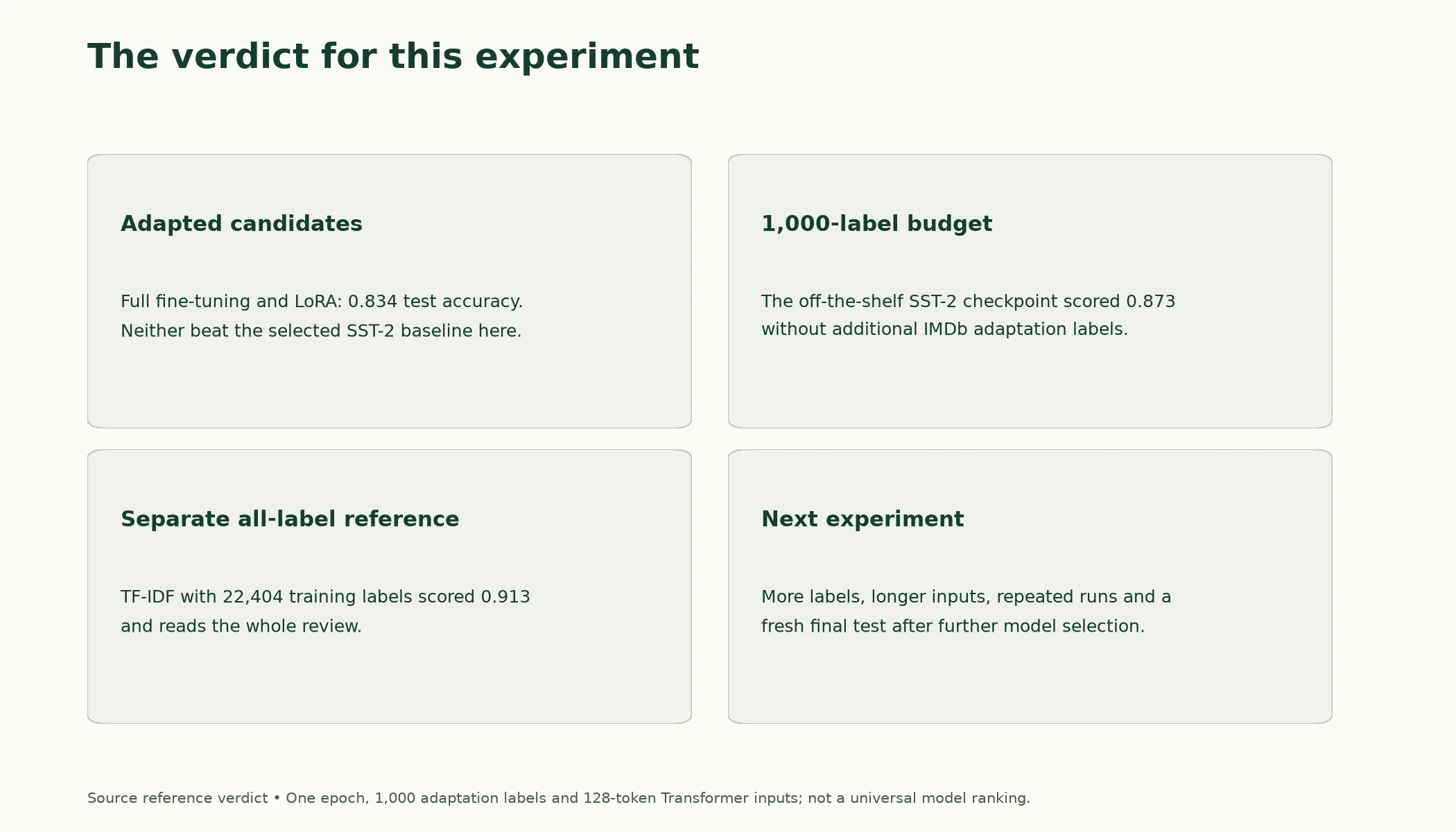
Figure 8.7.2. Keep/reject conclusions apply to the supplied one-epoch, 1,000-label experiment and declared requirements. Future tuning needs new validation work and a fresh final test sample.
Summary
- Evaluating an adapted model answers several questions: training behaviour, metrics with uncertainty, errors, overfitting and forgetting, comparison and cost, reproducibility, and the decision itself.
- All results files used the same split and the same 1,000 training reviews (checked by fingerprint).
- Training curves: loss fell from about ln 2 to 0.436 and 0.440 in the two runs; validation accuracy peaked at step 48. Validation loss wasn't recorded and should be next time.
- Metrics with 95% intervals: full fine-tuning and LoRA both 0.834 (0.810–0.856); SST-2 off the shelf 0.873 (0.851–0.892); TF-IDF with all labels 0.913 (0.894–0.929).
- Error analysis: the fine-tuned models shared 112 of 166 errors; methods reading 128 tokens dropped on long reviews; positive reviews full of negative words fooled the fine-tuned models but not the SST-2 model.
- Overfitting signs: validation-to-test drops of 0.013–0.046 (LoRA largest). Forgetting: 4.07 for full fine-tuning against 3.461 for LoRA (pretrained 3.381).
- Comparison: more trained parameters on the same 1,000 labels didn't help; every 1,000-label method was significantly worse than the off-the-shelf SST-2 model; only TF-IDF with all labels beat it.
- Variation: five TF-IDF training draws ranged 0.840–0.859 on validation. Results were tracked in
results/experiments.csv. - Decision, by rules set in advance: reject both adapted models; use the SST-2 model (or TF-IDF with all labels). The decision record lists limitations and next steps.
Glossary
| Term | Meaning |
|---|---|
| Training loss | Loss on the training batches. |
| Validation loss / accuracy | Loss or accuracy on held-out data, used to monitor generalisation. |
| Confidence interval | An interval from a method designed to cover the target quantity at a stated rate over repeated samples; this is not a probability assigned to the fixed unknown value. |
| Wilson interval | A standard confidence interval for a proportion. |
| Error analysis | Examining which examples a model gets wrong and why. |
| Error overlap | The number of errors two models share. |
| Validation–test gap | The drop from validation to test score, partly due to selecting on validation. |
| Paired sign test | Comparing two models on the same examples by counting where only one is right. |
| Run-to-run variation | Differences between runs caused by randomness. |
| Experiment tracking | Recording each run's settings, data, versions and results. |
| Keep-or-reject rule | A criterion, set in advance, for adopting a model. |
| Decision record | A written record of a decision with its evidence, limitations and next steps. |
Wrap-up
Quick check
What must be checked before combining result files?
Their provenance and aligned evaluation identities.
Does one retention probe measure every old capability?
No; it tests a specific setup and requires careful interpretation.
What follows further selection using the reported test data?
Evaluate the new choice on a fresh final test.
Questions and discussion
Ask about this lesson, share what you found in a lab, or help someone else. Posts are public on the course's GitHub Discussions: anyone can read them, and you need a GitHub account to post.
Opening it loads giscus from giscus.app.