Overfitting, and What to Do About It
- Time
- ~80 min
- Sections
- 10
- Code cells
- 21
- Labs
- 5
- Figures
- 5
Before you start
A network that is too big for its data memorises it. You make that happen on purpose (German Credit: 500 training rows,
48,897 parameters, training AUC 1.0 and a validation loss 3.4 times worse than its best), learn why validation loss and AUC
tell different stories (confidence against ranking), and compare the four standard fixes: a smaller model, weight decay,
dropout (plus the model.eval() bug) and early stopping. Then the twist: once early stopping is applied, every
configuration lands within the noise floor of a 250-row validation set. Measure the noise before you believe a ranking.
- Learning goal
Lesson 3.1 made the network learn quickly. This notebook studies the opposite failure: a network can become very good at reproducing the training data while becoming worse at making predictions on new data. That failure is called overfitting.
The central question is not simply, “How do I stop overfitting?” It is:
How do I know that I am overfitting, what exactly is going wrong, and which intervention addresses that particular problem?
You will deliberately create overfitting, learn to recognise it from both loss and metric curves, and then compare four standard ways of controlling it: reducing model capacity, weight decay, dropout, and early stopping.
One more idea is especially important: a validation result contains noise. A configuration that scores 0.01 higher on one validation split has not automatically improved the model. You need to know how much the score naturally moves when the data changes slightly.
By the end, you should be able to:
- recognise overfitting from training/validation curves;
- explain what model capacity means and why it interacts with dataset size;
- distinguish what validation loss measures from what ROC-AUC measures;
- explain what each regularisation method actually changes;
- recognise both under-regularisation and over-regularisation;
- measure the noise in your validation result before treating a small difference as an improvement.
- You will be able to
- Explain why the amount of training data, relative to model capacity, determines whether serious memorisation is possible.
- Produce overfitting deliberately and identify it from both loss and metric curves.
- Explain why validation loss and validation AUC can tell different stories.
- Compare four interventions: reduced capacity, weight decay, dropout, and early stopping.
- Recognise the characteristic signs of over-regularisation.
- Measure the variability of your own validation set and use that measurement when interpreting close results.
Why 45,000 rows cannot teach this
Before swapping datasets, let's test the reason for the swap.
The problem we want to study is overfitting: a model having enough flexibility to fit details that are specific to its training examples rather than details that generalise to new examples.
A useful first diagnostic is the relationship between model capacity and amount of training data.
- A parameter is a trainable number in the model, such as a weight or bias.
- Model capacity is the model's ability to represent different functions. More parameters often give a model more capacity, although parameter count is only a rough proxy for capacity.
- A training example is one row the model is allowed to learn from.
If there are vastly more training examples than parameters, the model has relatively little room to give every individual row its own special treatment. It is pushed towards finding patterns shared across many examples.
If there are many more parameters than training examples, the model has much more freedom. It can potentially fit individual examples or small groups of examples instead of learning only the broad structure.
So parameters per training example is a useful diagnostic here, not a law of machine learning. The experiment below measures it for the Module 2 setup rather than assuming that the ratio alone determines whether overfitting will occur.
# Rebuild the Module 2 Bank Marketing setup just far enough to measure it.DATA_DIR = "data"; os.makedirs(DATA_DIR, exist_ok=True)CSV = os.path.join(DATA_DIR, "bank-full.csv")if not os.path.exists(CSV): url = "https://archive.ics.uci.edu/static/public/222/bank+marketing.zip" raw = urllib.request.urlopen(url, timeout=120).read() outer = zipfile.ZipFile(io.BytesIO(raw)) inner = zipfile.ZipFile(io.BytesIO(outer.read("bank.zip"))) open(CSV, "wb").write(inner.read("bank-full.csv"))bm = pd.read_csv(CSV, sep=";")bm_y = (bm["y"] == "yes").astype(np.float32).valuesbm_X = bm.drop(columns=["y", "duration"])bnum = bm_X.select_dtypes(include="number").columns.tolist()bcat = [c for c in bm_X.columns if c not in bnum]bXtr, bXva, bytr, byva = train_test_split(bm_X, bm_y, test_size=0.2, random_state=SEED, stratify=bm_y)bpre = ColumnTransformer([("n", StandardScaler(), bnum), ("c", OneHotEncoder(handle_unknown="ignore", sparse_output=False), bcat)])bA = bpre.fit_transform(bXtr).astype(np.float32); bV = bpre.transform(bXva).astype(np.float32)bm_params = 50*64+64 + 64*32+32 + 32*1+1print(f"Bank Marketing : {bA.shape[0]:,} train rows, {bm_params:,} parameters " f"-> {bm_params/bA.shape[0]:.3f} parameters per training example")Bank Marketing : 36,168 train rows, 5,377 parameters -> 0.149 parameters per training example
# Train the Module 2 model far past its useful life and watch for memorisation.bXt = torch.tensor(bA); bYt = torch.tensor(bytr).unsqueeze(1)bXv = torch.tensor(bV); bYv = torch.tensor(byva).unsqueeze(1)torch.manual_seed(SEED)bmodel = nn.Sequential(nn.Linear(bA.shape[1],64), nn.ReLU(), nn.Linear(64,32), nn.ReLU(), nn.Linear(32,1))bopt = torch.optim.AdamW(bmodel.parameters(), lr=1e-3)bl = torch.utils.data.DataLoader(torch.utils.data.TensorDataset(bXt,bYt), batch_size=256, shuffle=True, generator=torch.Generator().manual_seed(SEED))bm_hist=[]t0=time.time()for ep in range(1, 41): bmodel.train() for xb,yb in bl: bopt.zero_grad(); loss_fn(bmodel(xb),yb).backward(); bopt.step() bmodel.eval() with torch.no_grad(): a=bmodel(bXt); b=bmodel(bXv) bm_hist.append(dict(ep=ep, trl=loss_fn(a,bYt).item(), vl=loss_fn(b,bYv).item(), tra=roc_auc_score(bytr,torch.sigmoid(a).numpy()), va=roc_auc_score(byva,torch.sigmoid(b).numpy())))print(f"40 epochs in {time.time()-t0:.0f}s")print(f"{'epoch':>6}{'train loss':>12}{'val loss':>10}{'train AUC':>11}{'val AUC':>9}{'gap':>8}")for x in bm_hist: if x["ep"] in (1,5,10,20,30,40): print(f"{x['ep']:>6}{x['trl']:>12.4f}{x['vl']:>10.4f}{x['tra']:>11.4f}{x['va']:>9.4f}{x['tra']-x['va']:>8.4f}")40 epochs in 3s
epoch train loss val loss train AUC val AUC gap
1 0.3105 0.3084 0.7595 0.7666 -0.0071
5 0.2892 0.2921 0.7945 0.7874 0.0070
10 0.2804 0.2879 0.8087 0.7927 0.0160
20 0.2709 0.2881 0.8258 0.7944 0.0314
30 0.2635 0.2902 0.8370 0.7911 0.0458
40 0.2575 0.2959 0.8471 0.7859 0.0612
There it is, measured rather than asserted.
After forty epochs — far more than anyone would normally need for this small demonstration — a gap opens between training and validation AUC, and validation AUC peaks and then drifts down slightly. So the Bank Marketing model does show some overfitting.
But notice the scale of the effect. Training loss is still around 0.26 rather than approaching zero, and training AUC is still well below 1.0. The model has not memorised the training rows in the way we are about to make the German Credit model memorise its 500 rows.
The parameter-to-example ratio helps explain why. The Bank Marketing model has roughly 0.15 parameters per training example. That does not make memorisation mathematically impossible in every sense, but it gives this particular network far less capacity per example than the German Credit experiment.
This matters for teaching and for experiments generally:
A method cannot look useful if the problem it is designed to solve is barely present.
If we added dropout to the Bank Marketing experiment and saw almost no change, that would not prove that dropout is useless. It would mostly tell us that this experiment is a poor place to demonstrate its effect.
The broader engineering lesson is even more important. Before evaluating a regulariser, architecture, optimiser, or other intervention, first establish that the failure mode it is supposed to address can actually be observed in your experiment.
Why is Bank Marketing a poor dataset for demonstrating dropout?
A method cannot look useful if the problem it addresses is barely present. First establish that the failure mode exists in your experiment.
State the general engineering lesson from Section 1 in your own words.
- Before evaluating a regulariser (or any intervention), confirm that the failure it targets is actually observable in your experiment.
- Otherwise 'no effect' tells you about the experiment, not about the method.
German Credit through the Module 2 pipeline
The dataset is changing; the basic modelling pipeline should not.
This is an important experimental principle: change one major thing at a time when you want to understand causality. Here we keep the preprocessing, tensor construction, MLP pattern, and training-loop structure familiar from Module 2, while changing the dataset and deliberately using a much smaller training set.
A few terms used in the code:
ColumnTransformerapplies different preprocessing to different groups of columns.StandardScalerstandardises numeric features.OneHotEncoderconverts categorical values into indicator columns.TensorDatasetpackages tensors so they can be consumed by a PyTorchDataLoader.- The training set is used to fit the model.
- The validation set is used to make development choices such as model size or when to stop.
- The test set is held back until the end so it can provide a less biased estimate of performance.
The preprocessing is fitted on the training data only. That prevents information from the validation or test rows from influencing the transformation learned from the training set.
gc = fetch_openml("credit-g", version=1, as_frame=True)X_raw = gc.data.copy()y_raw = (gc.target == "bad").astype(np.float32).values # positive class = bad credit riskgnum = X_raw.select_dtypes(include="number").columns.tolist()gcat = [c for c in X_raw.columns if c not in gnum]print(f"rows {X_raw.shape[0]} numeric {len(gnum)} categorical {len(gcat)}")print(f"class balance: bad {y_raw.mean():.3f} / good {1-y_raw.mean():.3f}")rows 1000 numeric 7 categorical 13 class balance: bad 0.300 / good 0.700
# 3-way split: 500 train / 250 val / 250 testX_tr_r, X_tmp, y_tr, y_tmp = train_test_split(X_raw, y_raw, train_size=500, random_state=SEED, stratify=y_raw)X_va_r, X_te_r, y_va, y_te = train_test_split(X_tmp, y_tmp, test_size=0.5, random_state=SEED, stratify=y_tmp)pre = ColumnTransformer([("n", StandardScaler(), gnum), ("c", OneHotEncoder(handle_unknown="ignore", sparse_output=False), gcat)])A_tr = pre.fit_transform(X_tr_r).astype(np.float32) # fit on TRAIN onlyA_va = pre.transform(X_va_r).astype(np.float32)A_te = pre.transform(X_te_r).astype(np.float32)D = A_tr.shape[1]Xt = torch.tensor(A_tr); Yt = torch.tensor(y_tr).unsqueeze(1)Xv = torch.tensor(A_va); Yv = torch.tensor(y_va).unsqueeze(1)Xs = torch.tensor(A_te); Ys = torch.tensor(y_te).unsqueeze(1)print(f"\ntrain {A_tr.shape} val {A_va.shape} test {A_te.shape}")print(f"majority-class accuracy on val: {max(y_va.mean(), 1-y_va.mean()):.4f}")print(f"majority-class accuracy on test: {max(y_te.mean(), 1-y_te.mean()):.4f}")train (500, 61) val (250, 61) test (250, 61) majority-class accuracy on val: 0.7000 majority-class accuracy on test: 0.7000
# The same MLP shape as Module 2, now sized for this feature count.def make_mlp(hidden=(256,128), p_drop=0.0, seed=SEED, d_in=None): """Build an MLP of any width and depth, with optional dropout, from reproducible weights. Each hidden size adds ``Linear → ReLU`` (plus ``Dropout`` when ``p_drop > 0``); a final ``Linear`` produces one logit. PyTorch is seeded first, so the same arguments always give the same initial weights. Args: hidden: Width of each hidden layer, in order, e.g. ``(256, 128)``. p_drop: Dropout probability after each hidden activation; 0 adds no dropout layers. seed: Seed for the weight initialisation. d_in: Number of input features; defaults to ``D``, the encoded German Credit width. Returns: An ``nn.Sequential`` that outputs one raw logit per row. """ torch.manual_seed(seed) d_in = d_in or D layers, prev = [], d_in for h in hidden: layers += [nn.Linear(prev, h), nn.ReLU()] if p_drop > 0: layers.append(nn.Dropout(p_drop)) prev = h layers.append(nn.Linear(prev, 1)) return nn.Sequential(*layers)def n_params(m): """Count the parameters of a model. Args: m: Any ``nn.Module``. Returns: The total number of elements across ``m.parameters()``. """ return sum(p.numel() for p in m.parameters())big = make_mlp()print(f"features {D}")print(f"model {str((256,128)):<12} {n_params(big):,} parameters")print(f"parameters per training row {n_params(big)/len(A_tr):.1f}")print()print(f"compare Bank Marketing: {bm_params/bA.shape[0]:.3f} parameters per training row")print(f"ratio: {(n_params(big)/len(A_tr)) / (bm_params/bA.shape[0]):,.0f}x more capacity per example")features 61 model (256, 128) 48,897 parameters parameters per training row 97.8 compare Bank Marketing: 0.149 parameters per training row ratio: 658x more capacity per example
Roughly a hundred parameters for every training row, compared with Bank Marketing's fraction of one. That is a very large change in capacity per training example, and we achieved it without introducing new modelling machinery.
The important phrase is “capacity per example.” It does not mean that every parameter stores one row. Neural networks do not work that way. It means that, relative to the amount of data available, the model has much more freedom to construct a complicated function.
That freedom makes memorisation possible. The next section deliberately pushes the model in that direction.
Two setups, 658 times apart
36,168 training rows, 5,377 parameters: 0.149 parameters per row. After 40 epochs: train AUC 0.847, validation 0.786.
500 training rows, 48,897 parameters: 97.8 parameters per row. After 60 epochs: train AUC 1.000, validation 0.742.
German Credit's model has about 98 parameters per training row, versus 0.15 for Bank Marketing. What does that mean?
'Capacity per example' is a rough diagnostic, not a law. Networks don't store rows one per parameter.
Why keep the Module 2 pipeline unchanged when switching datasets?
Changing several things at once makes it impossible to know what caused a difference.
Memorising 500 rows on purpose
Now we deliberately create the failure we want to study.
The model is large relative to the 500 training examples, and we train it for long enough without an explicit regularisation method. The purpose is not to build a useful credit model. The purpose is to make the difference between training performance and generalisation visible.
The key vocabulary:
- Training performance tells us how well the model fits examples it was allowed to learn from.
- Validation performance tells us how well that same model behaves on examples it did not train on.
- Generalisation means performing well on new examples drawn from the same underlying problem.
- Overfitting occurs when continued training improves the fit to the training data while performance on unseen data stops improving or gets worse.
Watch for the point where those two stories separate.
def run(hidden=(256,128), p_drop=0.0, wd=0.0, lr=1e-3, epochs=60, bs=32, seed=SEED, track_test=False): """Train one configuration for a fixed number of epochs and record both splits every epoch. Trains with AdamW on the 500 training rows, then after every epoch scores the whole training and validation sets in evaluation mode (loss, ROC-AUC, accuracy at 0.5). The weights with the lowest validation loss are copied, but training continues, so the history shows what happens after the best epoch. Args: hidden: Hidden-layer widths for ``make_mlp``. p_drop: Dropout probability. wd: Decoupled weight-decay coefficient for AdamW. lr: Learning rate. epochs: Number of epochs to train (no early stopping). bs: Mini-batch size. seed: Seed for the weights and the batch order. track_test: Also record test ROC-AUC every epoch (as ``"tea"``). Returns: A dict with ``"hist"`` (one record per epoch: ``trl``/``vl`` losses, ``tra``/``va`` AUCs, ``tracc``/``vacc`` accuracies), ``"best"`` (``vl``, ``epoch`` and ``state`` of the best-validation-loss epoch) and ``"model"`` (the model after the last epoch). """ model = make_mlp(hidden, p_drop, seed) opt = torch.optim.AdamW(model.parameters(), lr=lr, weight_decay=wd) g = torch.Generator().manual_seed(seed) loader = torch.utils.data.DataLoader(torch.utils.data.TensorDataset(Xt, Yt), batch_size=bs, shuffle=True, generator=g) hist, best = [], dict(vl=float("inf"), epoch=0, state=None) for ep in range(1, epochs+1): model.train() for xb, yb in loader: opt.zero_grad(); loss_fn(model(xb), yb).backward(); opt.step() model.eval() with torch.no_grad(): a, b = model(Xt), model(Xv) pa, pb = torch.sigmoid(a).numpy().ravel(), torch.sigmoid(b).numpy().ravel() rec = dict(ep=ep, trl=loss_fn(a, Yt).item(), vl=loss_fn(b, Yv).item(), tra=roc_auc_score(y_tr, pa), va=roc_auc_score(y_va, pb), tracc=accuracy_score(y_tr, pa > 0.5), vacc=accuracy_score(y_va, pb > 0.5)) if track_test: pc = torch.sigmoid(model(Xs)).numpy().ravel() rec["tea"] = roc_auc_score(y_te, pc) if rec["vl"] < best["vl"]: best = dict(vl=rec["vl"], epoch=ep, state=copy.deepcopy(model.state_dict())) hist.append(rec) return dict(hist=hist, best=best, model=model)One function trains every configuration in the lesson, records both splits every epoch, and remembers the best-validation-loss weights.
- 1
AdamW, so
wdis decoupled weight decay (Lesson 3.1). Withwd=0it is plain Adam. - 2
Score the whole training and validation sets in evaluation mode every epoch: 500 and 250 rows fit in one batch.
- 3
Accuracy needs a threshold; AUC and loss do not. Section 9 shows why that matters.
- 4
Keep a real copy of the best weights, but keep training: this function measures what happens after the best epoch.
The (256, 128) network trains for 60 epochs on 500 rows with no regularisation. Its validation loss is lowest early on. Where does it end up?
3.4 times its best: 0.4733 at epoch 5, 1.5925 at epoch 60, while training loss falls to 0.0006 and training AUC reaches 1.0. Validation AUC drops far less, from 0.82 to 0.74. Section 4 explains why the two disagree.
t0 = time.time()base = run()print(f"60 epochs on 500 rows: {time.time()-t0:.1f}s\n")h = base["hist"]print(f"{'epoch':>6}{'train loss':>12}{'val loss':>10}{'train AUC':>11}{'val AUC':>9}{'train acc':>11}")for x in h: if x["ep"] in (1,3,5,7,10,15,20,30,45,60): print(f"{x['ep']:>6}{x['trl']:>12.4f}{x['vl']:>10.4f}{x['tra']:>11.4f}{x['va']:>9.4f}{x['tracc']:>11.4f}")60 epochs on 500 rows: 0.4s
epoch train loss val loss train AUC val AUC train acc
1 0.5797 0.5893 0.7818 0.7154 0.7000
3 0.4755 0.4918 0.8429 0.8184 0.7560
5 0.4049 0.4733 0.8830 0.8095 0.8240
7 0.3302 0.5004 0.9236 0.7888 0.8700
10 0.2184 0.5745 0.9747 0.7640 0.9300
15 0.0707 0.7947 1.0000 0.7327 0.9980
20 0.0193 1.0120 1.0000 0.7381 1.0000
30 0.0043 1.2349 1.0000 0.7435 1.0000
45 0.0013 1.4542 1.0000 0.7422 1.0000
60 0.0006 1.5925 1.0000 0.7422 1.0000
fig, axes = plt.subplots(1, 2, figsize=(15, 5.3))eps = [x["ep"] for x in h]axes[0].plot(eps, [x["trl"] for x in h], label="train loss", color="#1b6ca8", lw=1.9)axes[0].plot(eps, [x["vl"] for x in h], label="val loss", color="#c1440e", lw=1.9)axes[0].axvline(base["best"]["epoch"], ls="--", c="0.4", lw=1.2, label=f"best val loss (ep {base['best']['epoch']})")axes[0].set_xlabel("epoch"); axes[0].set_ylabel("BCE loss"); axes[0].set_title("Loss")axes[1].plot(eps, [x["tra"] for x in h], label="train AUC", color="#1b6ca8", lw=1.9)axes[1].plot(eps, [x["va"] for x in h], label="val AUC", color="#c1440e", lw=1.9)axes[1].set_ylim(0.5, 1.02)axes[1].set_xlabel("epoch"); axes[1].set_ylabel("ROC-AUC"); axes[1].set_title("ROC-AUC")for a in axes: a.legend(fontsize=9); a.grid(alpha=0.3)plt.suptitle("(256,128) MLP, no regularisation, 500 training rows", y=1.02)plt.tight_layout(); plt.show()print(f"train AUC reaches {max(x['tra'] for x in h):.4f}")print(f"train accuracy reaches {max(x['tracc'] for x in h):.4f}")print(f"train loss falls to {min(x['trl'] for x in h):.6f}")print(f"val loss rises from {base['best']['vl']:.4f} (ep {base['best']['epoch']}) to {h[-1]['vl']:.4f} (ep 60)")print(f" -> val loss is {h[-1]['vl']/base['best']['vl']:.1f}x worse at the end than at its best")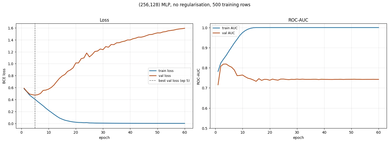
train AUC reaches      1.0000
train accuracy reaches 1.0000
train loss falls to    0.000595
val loss rises from    0.4733 (ep 5) to 1.5925 (ep 60)
  -> val loss is 3.4x worse at the end than at its best
This is textbook overfitting, and unlike Section 1 it took under three seconds to produce.
Training AUC reaches 1.0 — the model ranks all 500 training rows perfectly. Training loss also falls towards zero, which means the model is not merely getting the training labels right; it is becoming increasingly confident about them.
Meanwhile, validation loss reaches its minimum early and then climbs. Validation AUC also stops improving and begins to drift down.
The left panel shows the classic visual signature:
training and validation curves improve together at first; then the validation curve turns while the training curve continues improving.
That separation is the important event. The model is still becoming better at fitting the training examples, but those extra improvements are no longer transferring to unseen examples.
This is the distinction between fitting and generalising:
- fitting asks, “How well can I explain the examples I was given?”
- generalising asks, “How well does what I learned transfer to examples I have not seen?”
The model does not suddenly become incapable of learning after the turning point. It keeps learning — but increasingly learns details that are specific to the training set.
Now look at the right panel, because the metric there tells a different story.
Training loss keeps falling while validation loss has risen for 20 epochs. What is happening?
The model keeps learning, but increasingly learns details specific to the training set.
Explain the difference between 'fitting' and 'generalising' using what happened to the German Credit model.
- Fitting asks how well the model explains the examples it was given: training AUC reached 1.0 and training loss fell towards 0.
- Generalising asks how well that transfers to unseen rows: validation loss hit its minimum around epoch 5 and then more than tripled.
Two metrics, two stories
The loss panel says the model is becoming badly overconfident on validation data. The AUC panel says the deterioration in ranking is much smaller.
Both measurements are calculated from the same predictions on the same validation rows. The reason they disagree is that they measure different properties of those predictions.
Before deciding which curve to monitor, you need to understand exactly what each metric can and cannot see.
print(f"{'epoch':>6}{'val loss':>10}{'val AUC':>10}{'val acc':>10}")for x in h: if x["ep"] in (1,4,7,10,20,40,60): print(f"{x['ep']:>6}{x['vl']:>10.4f}{x['va']:>10.4f}{x['vacc']:>10.4f}")vl = [x["vl"] for x in h]; va = [x["va"] for x in h]print()print(f"val loss : best {min(vl):.4f} @ep{int(np.argmin(vl))+1} -> final {vl[-1]:.4f} " f"({100*(vl[-1]-min(vl))/min(vl):+.0f}%)")print(f"val AUC : best {max(va):.4f} @ep{int(np.argmax(va))+1} -> final {va[-1]:.4f} " f"({100*(va[-1]-max(va))/max(va):+.1f}%)") epoch val loss val AUC val acc
1 0.5893 0.7154 0.7000
4 0.4810 0.8187 0.7680
7 0.5004 0.7888 0.7240
10 0.5745 0.7640 0.7200
20 1.0120 0.7381 0.7640
40 1.3979 0.7423 0.7400
60 1.5925 0.7422 0.7400
val loss : best 0.4733 @ep5 -> final 1.5925 (+236%)
val AUC : best 0.8187 @ep4 -> final 0.7422 (-9.3%)
# Why they disagree: look at the predicted probabilities early vs late.early = make_mlp(); early.load_state_dict(base["best"]["state"]); early.eval()late = base["model"]; late.eval()with torch.no_grad(): p_early = torch.sigmoid(early(Xv)).numpy().ravel() p_late = torch.sigmoid(late(Xv)).numpy().ravel()fig, axes = plt.subplots(1, 2, figsize=(13, 3.8), sharey=True)for ax, p, tag in [(axes[0], p_early, f"best-val-loss checkpoint (ep {base['best']['epoch']})"), (axes[1], p_late, "final epoch (ep 60)")]: ax.hist(p[y_va==0], bins=30, alpha=0.65, label="actual: good", color="#1b6ca8") ax.hist(p[y_va==1], bins=30, alpha=0.65, label="actual: bad", color="#c1440e") ax.set_title(tag); ax.set_xlabel("predicted P(bad)"); ax.legend(fontsize=8)axes[0].set_ylabel("validation rows")plt.suptitle("Same ranking ability, wildly different confidence", y=1.03)plt.tight_layout(); plt.show()print(f"predictions above 0.99 or below 0.01:")print(f" early checkpoint: {((p_early>0.99)|(p_early<0.01)).mean():6.1%} of validation rows")print(f" final epoch : {((p_late >0.99)|(p_late <0.01)).mean():6.1%} of validation rows")print()print(f"mean predicted P(bad) for rows that are actually BAD:")print(f" early {p_early[y_va==1].mean():.3f} final {p_late[y_va==1].mean():.3f}")print(f"mean predicted P(bad) for rows that are actually GOOD:")print(f" early {p_early[y_va==0].mean():.3f} final {p_late[y_va==0].mean():.3f}")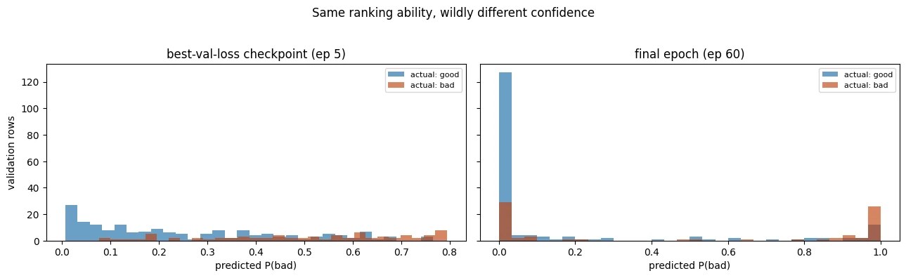
predictions above 0.99 or below 0.01:
  early checkpoint:   0.8% of validation rows
  final epoch     :  69.2% of validation rows

mean predicted P(bad) for rows that are actually BAD:
  early 0.508   final 0.498
mean predicted P(bad) for rows that are actually GOOD:
  early 0.247   final 0.155
Now the disagreement makes sense.
ROC-AUC: “Did I put the bad cases above the good cases?”
ROC-AUC measures ranking quality. Informally, it asks:
If I randomly choose one bad-credit row and one good-credit row, how often does the model assign the bad row a higher score?
Because AUC cares about the ordering of scores, it is largely insensitive to a transformation that preserves that ordering. For example, making predictions more extreme without changing their order can leave AUC unchanged.
Cross-entropy loss: “Were the predictions correct, and how confident were they?”
BCEWithLogitsLoss evaluates the quality of the predicted probabilities implied by the logits. A confident mistake is much more costly than a mistake made with moderate confidence.
For example, predicting 0.99 for an event that does not happen is treated much more harshly than predicting 0.60 for the same event.
That gives us two different questions:
- AUC: Are the risky cases generally ranked above the less risky cases?
- Loss: Are the predictions, including their confidence, compatible with the observed outcomes?
The overfitted model has therefore retained much of its ranking ability while becoming increasingly extreme in its predictions. That is why the AUC curve can look relatively stable while validation loss becomes much worse.
The histogram makes this visible: the final model pushes many predictions towards the extremes, while the earlier checkpoint keeps more predictions in the middle.
Which metric should you act on?
There is no universal answer. The correct metric depends on what the model's output is used for.
- If the output is used mainly for ranking or prioritisation — for example, reviewing the 100 highest-risk applications — AUC directly describes an important part of the task.
- If the output is used as a probability in an expected-loss calculation, threshold decision, or human-facing risk estimate, probability quality and calibration matter much more.
- If you are deciding when to stop training, validation loss can provide a useful stopping signal here because it reacts strongly to the overconfidence that appears after the best checkpoint.
The important habit is not “always use loss” or “always use AUC.” It is:
Know what failure modes your metric can see, and check another measurement for failures it cannot see.
-
Suppose a bug multiplies every output logit by 3 before the sigmoid. Which of validation AUC, validation loss, and validation accuracy would change, and which could remain unchanged? Explain your answer in terms of ranking, thresholding, and confidence.
Multiplying every logit by 3 keeps their order and their sign.
- ROC-AUC: unchanged. It depends only on how the rows are ordered, and a positive scaling preserves the order exactly.
- Accuracy at 0.5: unchanged. A row is predicted positive when \(\sigma(z) > 0.5\), which means \(z > 0\), and \(3z > 0\) exactly when \(z > 0\). The threshold sits at the one point scaling cannot move.
- Loss: changes. Every probability is pushed towards 0 or 1: confident correct predictions cost a little less and wrong ones cost much more. For a calibrated model the loss rises; for an under-confident model it could even fall.
In short: ranking and the 0.5 threshold are blind to the bug, confidence is not. (A bug that added a constant to the logits would also change accuracy, but still not AUC.) The lab above shows all three.
A bug multiplies every logit by 3 before the sigmoid. Which metric can stay exactly the same?
Multiplying by 3 preserves the order of the scores, so AUC is unchanged. The confidence changes, so the loss changes. Accuracy at 0.5 is also unchanged, because the sign of each logit is preserved.
Late in training, 69% of validation predictions were above 0.99 or below 0.01. What does that explain?
Confident mistakes are punished hard by the loss; AUC only sees the ordering.
Loss or AUC: which should you monitor? Give the lesson's answer, not a single metric.
- It depends on how the output is used: AUC for ranking/prioritisation; probability quality (loss, calibration) when outputs are used as probabilities or thresholded decisions.
- Know what failure modes each metric can see, and check another measurement for the failures it cannot (e.g. loss caught the overconfidence AUC missed).
Capacity first: the cheapest regulariser is a smaller model
Once you see overfitting, it is tempting to add dropout or weight decay immediately.
Start with the simplest question instead:
Do I actually need a model this large?
Section 2 showed that the model has much more capacity than the 500 training rows require. The most direct response to excess capacity is to reduce the capacity.
A smaller network has fewer trainable parameters and therefore fewer degrees of freedom. That can make it harder for the model to memorise individual training examples.
This is often called a regularisation effect: we are constraining the set of functions the model can represent so that solutions that fit arbitrary training-set details become harder to reach.
Capacity reduction is different from the other interventions in this notebook because it changes the model itself rather than adding a penalty or changing when training stops.
cap_runs = {}for hidden in [(256,128), (64,32), (16,8), (8,)]: r = run(hidden=hidden) cap_runs[hidden] = r hh = r["hist"] vl_ = [x["vl"] for x in hh]; va_ = [x["va"] for x in hh] print(f"{str(hidden):<12} params {n_params(make_mlp(hidden)):>7,} " f"best val loss {min(vl_):.4f}@{int(np.argmin(vl_))+1:>2} " f"best val AUC {max(va_):.4f} final val AUC {va_[-1]:.4f} " f"final train AUC {hh[-1]['tra']:.4f}")(256, 128) params 48,897 best val loss 0.4733@ 5 best val AUC 0.8187 final val AUC 0.7422 final train AUC 1.0000 (64, 32) params 6,081 best val loss 0.4706@10 best val AUC 0.8158 final val AUC 0.7253 final train AUC 1.0000 (16, 8) params 1,137 best val loss 0.4644@20 best val AUC 0.8244 final val AUC 0.7650 final train AUC 0.9552 (8,) params 505 best val loss 0.4569@37 best val AUC 0.8360 final val AUC 0.8163 final train AUC 0.8784
fig, axes = plt.subplots(1, 2, figsize=(13, 4.3))cols = plt.cm.viridis(np.linspace(0, 0.88, len(cap_runs)))for c, (hid, r) in zip(cols, cap_runs.items()): hh = r["hist"]; e = [x["ep"] for x in hh] axes[0].plot(e, [x["vl"] for x in hh], color=c, lw=1.9, label=str(hid)) axes[1].plot(e, [x["tra"]-x["va"] for x in hh], color=c, lw=1.9, label=str(hid))axes[0].set_ylabel("validation loss"); axes[0].set_title("Validation loss by capacity")axes[1].set_ylabel("train AUC − val AUC"); axes[1].set_title("Generalisation gap")axes[1].axhline(0, c="0.4", lw=1)for a in axes: a.set_xlabel("epoch"); a.legend(fontsize=9, title="hidden"); a.grid(alpha=0.3)plt.tight_layout(); plt.show()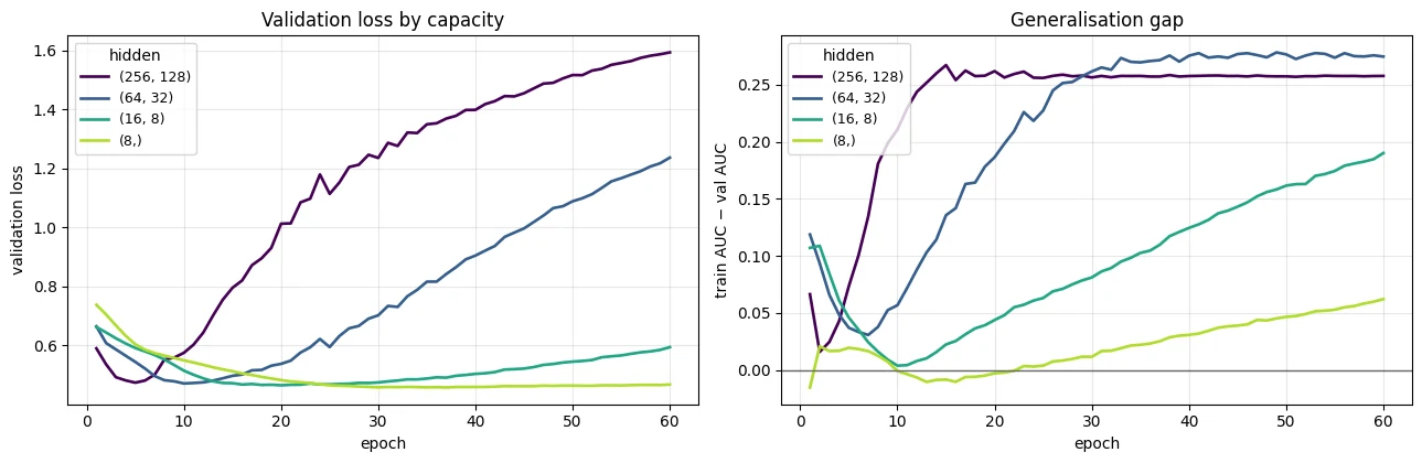
The trend in validation loss is monotone in this experiment: reducing capacity lowers the validation loss, with the smallest model performing best. Validation AUC is noisier — the (64,32) model is slightly below the largest model — which is our first warning that small numerical differences may be measurement noise rather than genuine improvements.
The clearer evidence is in the overfitting pattern. Shrinking the network greatly reduces the upward drift in validation loss and narrows the gap between training and validation behaviour. The smallest model never reaches a training AUC of 1.0, so it has not memorised the training set in the same way as the oversized network.
That does not, by itself, prove that the smallest model is perfect. A model can fail to reach training AUC of 1.0 for two very different reasons:
- it is appropriately constrained and is learning the useful structure; or
- it is too small to represent important structure in the problem.
This is the distinction between regularisation and underfitting. If we reduce capacity too far, both training and validation performance can suffer because the model is no longer expressive enough.
That is why capacity reduction is a useful first experiment: it is cheap, simple, and it tells us how much capacity the problem appears to need.
Why is a small model not always the answer? Some problems genuinely require large models. Images, language, and other high-dimensional tasks can contain structure that a tiny network simply cannot represent. In those settings, we may want to keep a large model while using constraints such as weight decay, dropout, data augmentation, or other methods to reduce harmful memorisation.
-
The smallest model here never reached training AUC of 1.0. Is that automatically evidence of underfitting? What additional evidence would you inspect to distinguish “too small” from “small enough”?
No. A training AUC below 1.0 only says the model cannot memorise the training set, which is what regularisation is for. Underfitting would show up as training and validation performance both low and close together, with validation improving when you add capacity. Evidence to inspect: the validation trend across sizes (here the
(8,)model has the lowest best validation loss, 0.4569, and the highest best validation AUC, 0.836); the gap between final training and validation AUC (about 0.06 for(8,), against 0.26 for the big model); learning curves over more epochs and more data (does more data help a small model?); and a simple baseline such as logistic regression. If a slightly larger model does not beat it on validation by more than the noise floor, the small model is small enough.
Which intervention removes capacity rather than constraining how it is used?
Fewer parameters mean fewer degrees of freedom. Weight decay and dropout keep the capacity but change which solutions training prefers.
The smallest model never reached training AUC 1.0. Is that automatically underfitting?
Regularisation and underfitting both stop memorisation. Underfitting also hurts validation, because the model can no longer express important structure.
Weight decay
Weight decay adds a pressure for model parameters to remain smaller during training.
The simple intuition is that very large weights can help a network create sharp, highly specific responses. A function that bends sharply to pass through many scattered training examples can require stronger parameter values than a smoother function that captures a broad pattern.
Weight decay therefore adds a preference for solutions with smaller parameter magnitudes.
In this notebook, the implementation uses AdamW, which applies weight decay in a way that is decoupled from Adam's gradient-based update. Lesson 3.1 covered that optimisation detail; here the important idea is the modelling effect:
Weight decay does not remove parameters. It makes large parameter values more costly to maintain.
That distinction matters when we compare it with reduced capacity in Section 5.
wd_runs = {}for wd in [0.0, 0.01, 0.1, 0.3, 1.0]: r = run(wd=wd); wd_runs[wd] = r hh = r["hist"]; vl_=[x["vl"] for x in hh]; va_=[x["va"] for x in hh] wnorm = torch.cat([p.detach().flatten() for p in r["model"].parameters()]).norm().item() print(f"wd={wd:<5} best val loss {min(vl_):.4f} final val loss {vl_[-1]:.4f} " f"best val AUC {max(va_):.4f} final train AUC {hh[-1]['tra']:.4f} ||w||={wnorm:7.2f}")wd=0.0 best val loss 0.4733 final val loss 1.5925 best val AUC 0.8187 final train AUC 1.0000 ||w||= 18.99 wd=0.01 best val loss 0.4733 final val loss 1.5646 best val AUC 0.8187 final train AUC 1.0000 ||w||= 18.91 wd=0.1 best val loss 0.4729 final val loss 1.4558 best val AUC 0.8189 final train AUC 1.0000 ||w||= 18.11 wd=0.3 best val loss 0.4727 final val loss 1.2625 best val AUC 0.8194 final train AUC 1.0000 ||w||= 16.89 wd=1.0 best val loss 0.4723 final val loss 0.9639 best val AUC 0.8202 final train AUC 1.0000 ||w||= 15.14
fig, axes = plt.subplots(1, 2, figsize=(15, 5.0))cols = plt.cm.plasma(np.linspace(0, 0.85, len(wd_runs)))for c,(wd,r) in zip(cols, wd_runs.items()): hh=r["hist"]; e=[x["ep"] for x in hh] axes[0].plot(e, [x["vl"] for x in hh], color=c, lw=1.8, label=f"wd={wd}")axes[0].set_ylabel("validation loss"); axes[0].set_title("Weight decay tames the loss blow-up")ws = [torch.cat([p.detach().flatten() for p in r["model"].parameters()]).norm().item() for r in wd_runs.values()]axes[1].bar([str(w) for w in wd_runs], ws, color="#1b6ca8")axes[1].set_xlabel("weight decay"); axes[1].set_ylabel("final ||w||")axes[1].set_title("...by actually shrinking the weights")axes[0].set_xlabel("epoch"); axes[0].legend(fontsize=9); axes[0].grid(alpha=0.3)plt.tight_layout(); plt.show()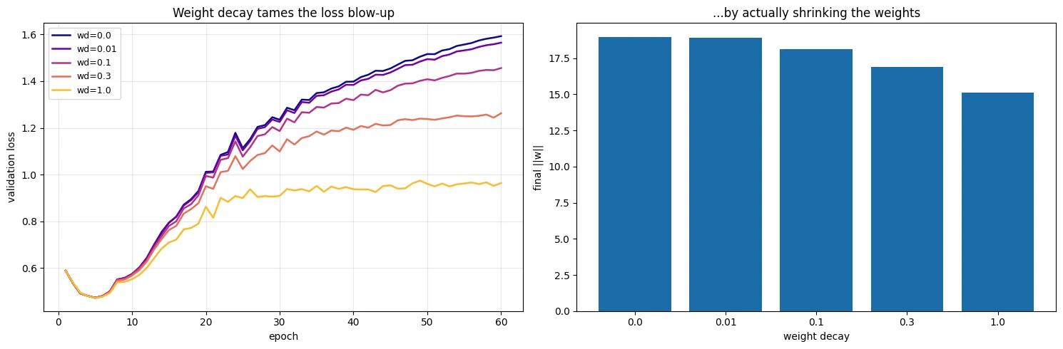
Weight decay does what the mechanism predicts: as the coefficient increases, the final weight norm falls, and the validation-loss blow-up becomes less severe.
A weight norm is a single number summarising the overall magnitude of the model's parameters. A lower norm therefore confirms that the regulariser is actually changing the parameter values, not merely producing a coincidental change in the validation curve.
Be precise about the result. At the strongest setting, the validation-loss blow-up is reduced, not eliminated. At the smaller coefficients, the effect is barely visible in this experiment.
The validation AUC also changes much less than the validation loss. That is understandable from Section 4: weight decay is affecting the confidence and shape of the learned function, while AUC only cares about the ordering of predictions.
So the correct conclusion is not “weight decay improves AUC” or “weight decay does nothing.” The more precise conclusion is:
In this experiment, weight decay strongly changes parameter magnitude and reduces loss deterioration, while its effect on ranking quality is comparatively small.
Notice another important difference from Section 5. The models can still reach training AUC of 1.0. Weight decay has not removed the model's capacity; it has changed which parameter configurations the optimiser prefers.
Reduced capacity: remove some of the model's ability to represent complicated functions.
Weight decay: keep the capacity, but discourage solutions that require large weights.
That distinction is worth remembering because the two methods can produce similar-looking improvements for different reasons.
How do you confirm that weight decay is actually changing the model, not coincidentally changing a curve?
The mechanism predicts smaller weights. A falling \(\|w\|\) shows the regulariser is doing what it claims.
Contrast reduced capacity and weight decay in one sentence each.
- Reduced capacity removes some of the model's ability to represent complicated functions (fewer parameters).
- Weight decay keeps the capacity but makes large parameter values costly, steering the optimiser towards smoother solutions (the model could still reach training AUC 1.0).
Dropout, and the bug everyone writes once
Dropout randomly sets some activations to zero during training.
An activation is the value produced by a neuron after its input has passed through the layer and activation function. With dropout, some of those values are temporarily removed on each training step.
This means the model cannot depend too heavily on any one unit being present. Across many updates it is encouraged to distribute useful information across multiple pathways instead of building a fragile solution that depends on a particular collection of units.
There is a crucial asymmetry:
- during training, dropout is active;
- during evaluation, dropout must be disabled.
PyTorch controls this behaviour through model.train() and model.eval().
This is not just a cosmetic switch. It changes the behaviour of layers such as Dropout and BatchNorm. Forgetting to call model.eval() before validation or testing can therefore make your reported metric noisy or systematically wrong.
We will deliberately create that bug before fixing it.
drop_runs = {}for p in [0.0, 0.2, 0.5, 0.8]: r = run(p_drop=p); drop_runs[p] = r hh=r["hist"]; vl_=[x["vl"] for x in hh]; va_=[x["va"] for x in hh] print(f"dropout={p:<4} best val loss {min(vl_):.4f} final val loss {vl_[-1]:.4f} " f"best val AUC {max(va_):.4f} final train AUC {hh[-1]['tra']:.4f}")dropout=0.0 best val loss 0.4733 final val loss 1.5925 best val AUC 0.8187 final train AUC 1.0000 dropout=0.2 best val loss 0.4652 final val loss 1.4917 best val AUC 0.8259 final train AUC 1.0000 dropout=0.5 best val loss 0.4553 final val loss 1.1959 best val AUC 0.8335 final train AUC 1.0000 dropout=0.8 best val loss 0.4548 final val loss 0.6066 best val AUC 0.8286 final train AUC 0.9794
# THE BUG: evaluating without model.eval()m = drop_runs[0.5]["model"]m.eval() # correctwith torch.no_grad(): p_correct = torch.sigmoid(m(Xv)).numpy().ravel()auc_correct = roc_auc_score(y_va, p_correct)m.train() # WRONG: dropout still active at eval timetorch.manual_seed(0)runs_buggy = []for trial in range(5): with torch.no_grad(): pb = torch.sigmoid(m(Xv)).numpy().ravel() runs_buggy.append(roc_auc_score(y_va, pb))m.eval()print(f"correct (model.eval()) : val AUC {auc_correct:.4f} — identical every time")print(f"buggy (model.train()): val AUC {' '.join(f'{a:.4f}' for a in runs_buggy)}")print(f" spread across 5 identical evaluations: " f"{max(runs_buggy)-min(runs_buggy):.4f} AUC")print(f" mean penalty: {auc_correct-np.mean(runs_buggy):+.4f} AUC")- 1
torch.no_grad()below does not help: it switches off gradients, not dropout. - 2
Seeded so the five buggy scores are reproducible; each pass still draws a different dropout mask.
correct (model.eval()) : val AUC 0.7426   — identical every time
buggy   (model.train()): val AUC 0.7139 0.7505 0.6999 0.7520 0.7086
                         spread across 5 identical evaluations: 0.0521 AUC
                         mean penalty: +0.0176 AUC
Two symptoms identify this bug, and both are worth remembering.
1. The evaluation score can be worse than it should be
If dropout is still active, the model is being evaluated with randomly removed activations. You are therefore not evaluating the deterministic full network you intend to deploy.
2. Repeating the same evaluation gives different results
This is the giveaway.
If you evaluate the same model on the same data twice and the predictions or metrics change, some stochastic training behaviour is probably still active. In this experiment, leaving the model in training mode leaves dropout switched on.
A good development check is therefore simple: evaluate twice. If identical inputs and identical model parameters produce different predictions when you expect deterministic evaluation, investigate the model mode and other sources of randomness.
The same train()/eval() discipline matters for BatchNorm. In training mode, BatchNorm uses statistics computed from the current batch; in evaluation mode, it uses the running statistics collected during training. Lesson 3.3 covers BatchNorm in detail.
The dropout results themselves show a moderate reduction in the validation-loss blow-up, especially at stronger dropout rates. The effect on AUC is comparatively small in this experiment.
-
A colleague reports 0.84 AUC during training but 0.81 after reloading the checkpoint in a separate evaluation script, and the model contains dropout. Give two possible explanations — one involving
model.eval(), and one that does not — and describe the single check that would distinguish them.Involving
model.eval(): the evaluation script never callsmodel.eval(), so dropout is still active. The score is lower and changes from run to run (Section 7 measured a mean penalty of 0.018 AUC and a 0.05 spread).Not involving it: the reloaded model or data is not the one that scored 0.84. Common causes: the checkpoint saved the last epoch rather than the best; the 0.84 was computed on a different split (or during training, on batches, with a different metric routine); or the evaluation script rebuilds the preprocessing, for example refitting the scaler or one-hot encoder on the evaluation data, so the features no longer mean what they meant in training.
The single check: evaluate the reloaded model twice on the same data. If the two results differ, something stochastic is still on (dropout in training mode). If they are identical and still 0.81, the difference lies in the checkpoint, the data or the preprocessing.
Write inverted dropout
In training mode, zero each value with probability p and scale the survivors by \(1/(1-p)\) so the expected value is unchanged. In
evaluation mode, return x untouched. rng is a NumPy random generator.
You evaluate the same model on the same data twice and get AUC 0.751 and 0.709. The most likely cause?
Deterministic evaluation should give identical numbers. Call model.eval(). BatchNorm also behaves differently between modes.
A colleague gets 0.84 AUC during training but 0.81 in a separate evaluation script, with dropout in the model. Give two possible explanations and one check that separates them.
- One: the evaluation script forgot
model.eval(), so dropout is active (or the training-time number was made in train mode). - Another: a different checkpoint (last instead of best), different data/preprocessing or a different split.
- Check: evaluate the same data twice in the script; if the numbers differ, randomness (dropout/train mode) is active.
Early stopping
Section 3 showed validation loss reaching its minimum early and getting worse when training continued.
Early stopping turns that observation into a training rule:
- monitor a validation metric;
- remember the best value seen so far;
- save the corresponding model parameters;
- stop training when the metric has failed to improve for a chosen number of epochs.
That waiting period is called patience.
Early stopping is different from dropout and weight decay because it does not directly change the model architecture or add a penalty to the training objective. It changes how long you train and which checkpoint you keep.
In this experiment, that matters because the model is capable of continuing to reduce training loss after validation performance has already peaked.
def train_early_stopping(hidden=(256,128), p_drop=0.0, wd=0.0, lr=1e-3, max_epochs=200, patience=10, bs=32, seed=SEED, verbose=True): """Train with early stopping on validation loss, restore the best weights, then score. Stops once validation loss has not improved by more than 1e-5 for ``patience`` epochs, loads the best epoch's weights, and reports validation and test ROC-AUC for that restored model. Args: hidden: Hidden-layer widths for ``make_mlp``. p_drop: Dropout probability. wd: Decoupled weight-decay coefficient for AdamW. lr: Learning rate. max_epochs: Upper limit on epochs. patience: Epochs without improvement before stopping. bs: Mini-batch size. seed: Seed for the weights and the batch order. verbose: Print a line when training stops early. Returns: A dict with the restored ``"model"``, ``"best_epoch"``, ``"best_vl"`` (its validation loss), ``"val_auc"``, ``"test_auc"`` and ``"ran"`` (epochs actually run). """ model = make_mlp(hidden, p_drop, seed) opt = torch.optim.AdamW(model.parameters(), lr=lr, weight_decay=wd) g = torch.Generator().manual_seed(seed) loader = torch.utils.data.DataLoader(torch.utils.data.TensorDataset(Xt, Yt), batch_size=bs, shuffle=True, generator=g) best_vl, best_ep, best_state, since = float("inf"), 0, None, 0 for ep in range(1, max_epochs+1): model.train() for xb, yb in loader: opt.zero_grad(); loss_fn(model(xb), yb).backward(); opt.step() model.eval() with torch.no_grad(): vl = loss_fn(model(Xv), Yv).item() if vl < best_vl - 1e-5: best_vl, best_ep, since = vl, ep, 0 best_state = copy.deepcopy(model.state_dict()) # RESTORE the best, don't just stop else: since += 1 if since >= patience: if verbose: print(f" stopped at epoch {ep}: no improvement for {patience} epochs") break model.load_state_dict(best_state) # <- the step people forget model.eval() with torch.no_grad(): va = roc_auc_score(y_va, torch.sigmoid(model(Xv)).numpy().ravel()) te = roc_auc_score(y_te, torch.sigmoid(model(Xs)).numpy().ravel()) return dict(model=model, best_epoch=best_ep, best_vl=best_vl, val_auc=va, test_auc=te, ran=ep)print("early stopping, big unregularised model:")es_big = train_early_stopping()print(f" ran {es_big['ran']} epochs, restored epoch {es_big['best_epoch']}")print(f" val loss {es_big['best_vl']:.4f} val AUC {es_big['val_auc']:.4f} test AUC {es_big['test_auc']:.4f}")print()print("compare: same model trained a fixed 60 epochs with no early stopping")final_model = base["model"]; final_model.eval()with torch.no_grad(): print(f" val loss {base['hist'][-1]['vl']:.4f} val AUC {base['hist'][-1]['va']:.4f} " f"test AUC {roc_auc_score(y_te, torch.sigmoid(final_model(Xs)).numpy().ravel()):.4f}")- 1
Only an improvement larger than 1e-5 counts (a
min_delta), so rounding noise cannot reset patience. - 2
Ten epochs without improvement: stop.
- 3
Without this line you would report the model from the stopping epoch, ten epochs past the best.
- 4
The test score is computed once, after every decision, and never used to choose anything.
early stopping, big unregularised model:
  stopped at epoch 15: no improvement for 10 epochs
  ran 15 epochs, restored epoch 5
  val loss 0.4733  val AUC 0.8095  test AUC 0.7528

compare: same model trained a fixed 60 epochs with no early stopping
  val loss 1.5925  val AUC 0.7422  test AUC 0.7017
Three details in the implementation matter more than the basic concept.
1. Restore the best weights — do not merely stop
Suppose the best validation loss occurred at epoch 12 and your patience is 5. If you simply stop at epoch 17, you are holding the model from epoch 17, not the model that achieved the best validation result.
load_state_dict(best_state) restores the parameters from the best checkpoint.
So early stopping is really two operations:
choose when training should stop + keep the best model found before stopping.
2. Patience must be large enough for normal validation noise
Validation loss does not necessarily improve smoothly every epoch. A small upward movement can happen even while the overall trend is improving.
A patience of 1 reacts to every small upward fluctuation. A patience of 10 requires the model to fail to improve for a much longer period before stopping.
The correct patience therefore depends partly on how noisy your validation measurement is.
3. Early stopping uses the validation set for model selection
The validation set is no longer a neutral measurement if you repeatedly use it to choose among checkpoints.
For example, if you inspect 200 checkpoints and keep the one with the best validation AUC, the final validation AUC is optimistic: you selected the checkpoint partly because that particular validation set liked it.
That is why this notebook keeps a separate test set. The test set is not used to choose the model or stopping point. It is held back for the final measurement.
This distinction becomes part of the experimental protocol in Module 4.
-
Early stopping is sometimes described as “a regulariser that costs nothing.” Given the validation-set issue above, what does it actually cost? And if the validation set had only 30 rows, would you trust it to choose between 200 checkpoints? Explain why.
It costs data and honesty. Data: the validation rows cannot be used for training, and because the validation set now makes a decision, you need yet another untouched test set to report a fair number, so fewer rows are left to learn from. Honesty: the chosen checkpoint's validation score is optimistic, because it was picked for being the best on those rows. It also costs an evaluation every epoch, a copy of the best weights in memory, and two new settings (patience,
min_delta).Not with 30 rows. At a 30% positive rate that is about 9 bad and 21 good rows. The AUC of such a set moves by about 0.09 from one sample to the next (a simulation with this lesson's AUC), far more than the real differences between checkpoints. Choosing the best of 200 checkpoints would mostly choose the luckiest noise, and its score would be badly inflated. A bigger validation set, or cross-validation, is the fix.
Early stopping stops at epoch 15 with patience 10. Which weights should you keep?
Early stopping is two operations: decide when to stop, and restore the best model found before stopping.
Why is the validation score of the selected checkpoint mildly optimistic?
Selection benefits from luck on that set, which is why a separate test set stays untouched.
Over-regularising, and how much noise your validation set has
Every regularisation method has a strength setting, and pushing that setting too far can create a different problem: over-regularisation.
Over-regularisation means the constraints have become strong enough that the model is no longer free to represent useful structure.
The visual pattern is often the opposite of ordinary overfitting:
- the model is constrained enough that it cannot fit the training data as closely;
- useful signal can be suppressed;
- both training and validation performance can suffer.
There is a second issue here that is easy to miss: validation measurements are noisy.
If two configurations differ by 0.005 AUC, that difference might be real — or it might simply be caused by which rows happened to be placed in the validation set.
This section therefore asks two questions:
- What does over-regularisation look like?
- How large does a validation difference need to be before we should take it seriously?
over = run(hidden=(16,8), p_drop=0.8, wd=1.0)hh = over["hist"]print("aggressively regularised: (16,8), dropout 0.8, weight decay 1.0")print(f" best val AUC {max(x['va'] for x in hh):.4f} <- looks GOOD")print(f" best val loss {min(x['vl'] for x in hh):.4f}")print(f" final train AUC {hh[-1]['tra']:.4f} <- no memorisation at all")print(f" final val accuracy {hh[-1]['vacc']:.4f}")print(f" majority-class acc {max(y_va.mean(), 1-y_va.mean()):.4f} <- compare the two lines above")print()m = over["model"]; m.eval()with torch.no_grad(): p = torch.sigmoid(m(Xv)).numpy().ravel()print(f" predicted P(bad): min {p.min():.3f} max {p.max():.3f} mean {p.mean():.3f}")print(f" predictions above 0.5: {(p>0.5).sum()} out of {len(p)}")print()print(" For comparison, the tiny-but-not-over-regularised (8,) model:")t8 = cap_runs[(8,)]["hist"]print(f" best val AUC {max(x['va'] for x in t8):.4f} best val loss {min(x['vl'] for x in t8):.4f} " f"final val acc {t8[-1]['vacc']:.4f}")aggressively regularised: (16,8), dropout 0.8, weight decay 1.0
best val AUC 0.8424 <- looks GOOD
best val loss 0.5514
final train AUC 0.8408 <- no memorisation at all
final val accuracy 0.7000
majority-class acc 0.7000 <- compare the two lines above
predicted P(bad): min 0.193 max 0.448 mean 0.331
predictions above 0.5: 0 out of 250
For comparison, the tiny-but-not-over-regularised (8,) model:
best val AUC 0.8360 best val loss 0.4569 final val acc 0.7440
Here is the trap.
The over-regularised model has the highest best validation AUC in this notebook. If AUC were the only number you looked at, you might conclude that it is the best model.
But the rest of the evidence says something important. Its validation accuracy has collapsed to approximately the majority-class rate, and its predicted probabilities are compressed into a narrow range that rarely crosses the 0.5 decision threshold.
This exposes another limitation of AUC.
AUC is threshold-free: it evaluates how well the model orders examples across possible thresholds. It does not tell you whether a particular threshold, such as 0.5, will produce useful decisions.
So this model can still rank bad-credit cases above good-credit cases reasonably well while producing almost no positive classifications at the chosen threshold.
Compare this with Section 4:
- the overfitted model became too confident while retaining much of its ranking ability;
- the over-regularised model became too cautious while also retaining reasonable ranking ability.
AUC does not directly reveal either calibration problem.
The broader lesson is:
A metric can be excellent at measuring one property while being completely blind to another property you care about.
Now we reach the question that should sit behind every comparison in this notebook:
How large does a difference have to be before we can reasonably treat it as evidence of an improvement?
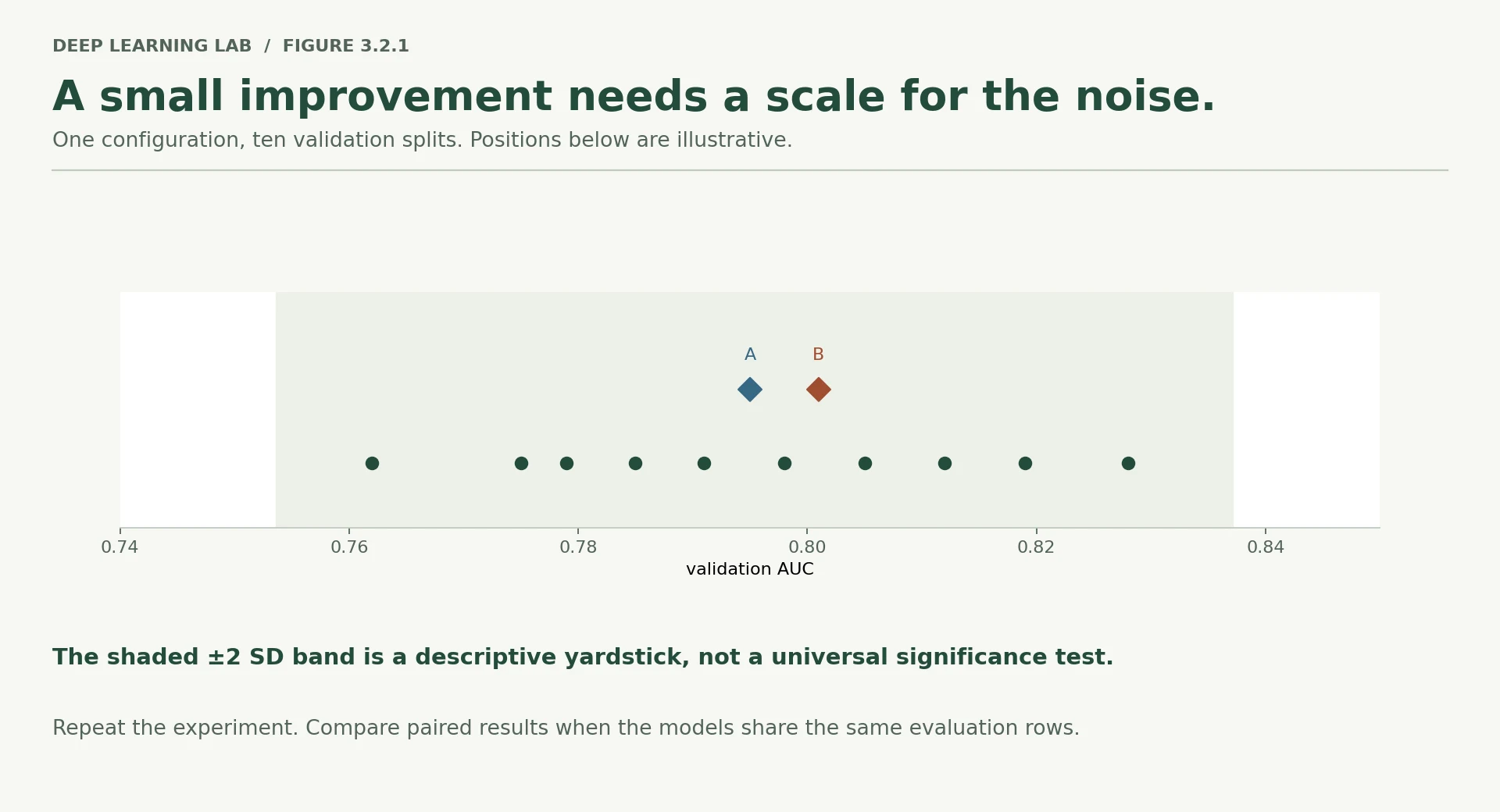
# Measure the noise floor: same config, same seed, only the data split changes.noise_aucs = []for rs in range(10): Xa, Xb_, ya, yb_ = train_test_split(X_raw, y_raw, train_size=500, random_state=rs, stratify=y_raw) Xv2, _, yv2, _ = train_test_split(Xb_, yb_, test_size=0.5, random_state=rs, stratify=yb_) p2 = ColumnTransformer([("n", StandardScaler(), gnum), ("c", OneHotEncoder(handle_unknown="ignore", sparse_output=False), gcat)]) A1 = p2.fit_transform(Xa).astype(np.float32); A2 = p2.transform(Xv2).astype(np.float32) torch.manual_seed(SEED); g = torch.Generator().manual_seed(SEED) mm = nn.Sequential(nn.Linear(A1.shape[1],16), nn.ReLU(), nn.Linear(16,8), nn.ReLU(), nn.Linear(8,1)) oo = torch.optim.AdamW(mm.parameters(), lr=1e-3) T1 = torch.tensor(A1); Y1 = torch.tensor(ya).unsqueeze(1) dl = torch.utils.data.DataLoader(torch.utils.data.TensorDataset(T1,Y1), batch_size=32, shuffle=True, generator=g) for _ in range(20): mm.train() for xb,yb in dl: oo.zero_grad(); loss_fn(mm(xb),yb).backward(); oo.step() mm.eval() with torch.no_grad(): noise_aucs.append(roc_auc_score(yv2, torch.sigmoid(mm(torch.tensor(A2))).numpy().ravel()))noise_aucs = np.array(noise_aucs)print("IDENTICAL configuration and seed, 10 different train/val splits:")print(" " + " ".join(f"{a:.4f}" for a in noise_aucs))print()print(f" mean {noise_aucs.mean():.4f}")print(f" standard deviation {noise_aucs.std():.4f}")print(f" min to max spread {noise_aucs.max()-noise_aucs.min():.4f}")print()print(f" => a difference smaller than about {2*noise_aucs.std():.3f} AUC is not distinguishable")print(f" from noise with a validation set of this size.")Ten runs in which only random_state of the split changes: the model, seed, epochs and preprocessing recipe are identical.
- 1
A different 500/250 split each time; stratified, so the 30% bad rate is kept.
- 2
The preprocessing is refitted on each new training split, exactly as a real rerun would do.
- 3
Same initial weights and batch order every time, so the spread comes from the data split alone.
IDENTICAL configuration and seed, 10 different train/val splits:
  0.7777  0.7874  0.7721  0.7857  0.7928  0.7410  0.7789  0.7582  0.7899  0.7797

  mean                0.7763
  standard deviation  0.0151
  min to max spread   0.0517

  => a difference smaller than about 0.030 AUC is not distinguishable
     from noise with a validation set of this size.
That number should change how you read every table in this notebook.
The same model configuration and seed, evaluated on different validation splits, produces a noticeable spread in AUC. That spread is the noise floor of this measurement: the amount the reported score can move simply because the validation examples changed.
Two standard deviations are only a rough descriptive yardstick here, not a universal statistical significance test. But the practical message is clear: if the difference between two configurations is smaller than the normal variation of the measurement, the experiment has not established that one configuration is genuinely better.
This is why several close comparisons in Sections 6 and 7 should not be turned into confident rankings. The capacity effect in Section 5 is much larger and more consistent; many of the smaller dropout and weight-decay differences are within the range of ordinary validation variation.
Three habits follow:
- Measure your noise floor before tuning. Then you know what size of improvement your experiment can realistically resolve.
- Report variability, not only a single point. Repeat across splits or seeds when close comparisons matter.
- Be suspicious of small gains after many trials. If you try many configurations, one of them will often obtain an unusually good validation score by chance. Selecting that winner does not prove that the underlying configuration is better.
This is a central idea in empirical machine learning: measurement noise and selection can create apparent improvements even when the underlying models are equally good.
Module 4 turns these ideas into a more formal experimental protocol.
Deep diveHow much noise does a 250-row validation set really have?
The ten splits give a standard deviation of 0.015. Sampling theory suggests the pure sampling noise of a 250-row validation set is larger: simulating scores with this lesson's AUC and class balance on fresh, independent 250-row sets gives a spread of about 0.03 (about 0.016 for 1,000 rows, and 0.09 for 30 rows). Ten measurements only estimate a spread roughly, and these ten splits share part of their rows. Treat "0.03" as an order of magnitude, not a threshold: a 0.005 gain is noise here, and a 0.05 gain needs checking on more splits or seeds before you believe it.
Config A scores 0.824 and config B 0.818 on validation. The same config varies with SD 0.015 across splits. What can you conclude?
A 0.006 gap is far smaller than normal split-to-split variation (≈0.03 at two SDs). Measure the noise floor before tuning.
The heavily regularised model had the best validation AUC but accuracy equal to the majority class. Why?
AUC is threshold-free, so it cannot see this calibration failure.
What is a 'noise floor', and how should it change the way you read a results table?
- The amount a score moves just because the evaluation data changes (same config and seed, different splits: here SD ≈ 0.015 AUC).
- Differences smaller than that are not evidence; repeat over splits or seeds for close comparisons, and be suspicious of small wins after many trials.
What to reach for first
The final table brings the interventions together.
The important question is not “Which technique has the highest number?” Instead, read the table alongside the mechanisms and the measurement noise from Section 9.
The test set is included here because it has been kept separate from model selection. A test score is meaningful only to the extent that we have not repeatedly used the test set to choose the model.
configs = [ ("no regularisation, (256,128)", dict(hidden=(256,128))), ("weight decay 1.0", dict(hidden=(256,128), wd=1.0)), ("dropout 0.5", dict(hidden=(256,128), p_drop=0.5)), ("dropout 0.5 + wd 0.1", dict(hidden=(256,128), p_drop=0.5, wd=0.1)), ("smaller model (16,8)", dict(hidden=(16,8))), ("tiny model (8,)", dict(hidden=(8,))), ("(16,8) + dropout 0.3 + wd 0.1",dict(hidden=(16,8), p_drop=0.3, wd=0.1)), ("OVER-regularised (16,8) p.8 wd1", dict(hidden=(16,8), p_drop=0.8, wd=1.0)),]print(f"{'configuration':<34}{'val AUC':>9}{'test AUC':>10}{'val loss':>10}{'stop ep':>9}")print("=" * 72)table = []for name, kw in configs: r = train_early_stopping(verbose=False, **kw) table.append((name, r)) print(f"{name:<34}{r['val_auc']:>9.4f}{r['test_auc']:>10.4f}{r['best_vl']:>10.4f}{r['best_epoch']:>9}")print("-" * 72)print(f"{'majority-class baseline (AUC)':<34}{0.5:>9.4f}{0.5:>10.4f}")print()print(f"noise floor (2 sd, measured in section 9): {2*noise_aucs.std():.4f} AUC")best_test = max(table, key=lambda t: t[1]["test_auc"])within = [n for n, r in table if best_test[1]["test_auc"] - r["test_auc"] < 2*noise_aucs.std()]print(f"configurations statistically indistinguishable from the best on TEST: {len(within)} of {len(table)}")for n in within: print(f" - {n}")configuration val AUC test AUC val loss stop ep ======================================================================== no regularisation, (256,128) 0.8095 0.7528 0.4733 5 weight decay 1.0 0.8112 0.7544 0.4723 5 dropout 0.5 0.8288 0.7656 0.4553 7 dropout 0.5 + wd 0.1 0.8293 0.7659 0.4552 7 smaller model (16,8) 0.8192 0.7619 0.4644 20 tiny model (8,) 0.8278 0.7637 0.4569 37 (16,8) + dropout 0.3 + wd 0.1 0.8201 0.7685 0.4611 37 OVER-regularised (16,8) p.8 wd1 0.8288 0.7622 0.5338 88 ------------------------------------------------------------------------ majority-class baseline (AUC) 0.5000 0.5000 noise floor (2 sd, measured in section 9): 0.0302 AUC configurations statistically indistinguishable from the best on TEST: 8 of 8 - no regularisation, (256,128) - weight decay 1.0 - dropout 0.5 - dropout 0.5 + wd 0.1 - smaller model (16,8) - tiny model (8,) - (16,8) + dropout 0.3 + wd 0.1 - OVER-regularised (16,8) p.8 wd1
Read that last block of output carefully. The most important result is not a tidy ranking of regularisers.
Once early stopping is applied, the configurations in the final table are statistically indistinguishable within the resolution of this experiment on the untouched test set. The spread is smaller than the noise floor measured in Section 9.
That does not prove that the methods are universally equivalent. It means that this experiment, with this dataset, split, model family, seeds, and sample size, does not provide enough evidence to separate them reliably on the test measurement.
That distinction matters. “We cannot distinguish them here” is different from “they are mathematically identical.”
Deep diveComparing on the same test rows is a paired comparison
The noise floor was measured by changing the split. The final table scores every configuration on the same 250 test rows, and then much of the noise is shared: every model finds the same rows easy and the same rows hard. The quantity that matters is the noise of the difference between two models, which is usually well below either score's own spread. Bootstrapping the test rows and recomputing both AUCs on each resample gives that directly, and the same resamples give a confidence interval for the gap. So "8 of 8 within the noise floor" is a cautious reading. It is still the right conclusion for this lesson: no configuration has a margin you could defend.
What to take away
1. Overfitting requires enough freedom relative to the available data.
The Bank Marketing setup showed only mild overfitting in this experiment. German Credit, with only 500 training rows and a much larger model relative to the dataset, made the failure obvious.
Before choosing a fix, first establish that the failure mode exists.
2. Validation loss and validation AUC answer different questions.
Loss is sensitive to confidence as well as correctness. AUC focuses on ranking. The overfitted model stayed a useful ranker for longer than it remained a well-behaved probability estimator, while the over-regularised model could retain ranking ability while producing predictions that were too compressed for a 0.5 decision threshold.
3. Early stopping mattered strongly in this experiment.
With a fixed 60-epoch budget, capacity appeared to produce large differences because the larger models were allowed to continue past their useful checkpoints. When early stopping is applied, those differences largely disappear on the final test measurement.
So part of what the other regularisation methods appeared to accomplish was simply preventing the model from being trained beyond the point where validation performance was best.
That is a conclusion about this experiment, not a universal claim that early stopping makes every other regulariser unnecessary.
4. Restore the best weights.
Stopping at the end of the patience window is not enough. You must keep the parameters from the best validation checkpoint; otherwise you deliberately return to a later, worse model.
5. Measure the noise floor before trusting a ranking.
This is the habit that turns the notebook from a list of techniques into an experimental method.
If two configurations differ by less than the normal variability of your validation/test measurement, the honest conclusion may be that your experiment cannot yet tell them apart.
That is not a disappointing result. It is useful information about the resolution of your experiment.
The next step is to formalise that discipline: control the split, seeds, model-selection procedure, and final evaluation so that improvements are separated from noise.
Transition to Lesson 3.3
Lessons 3.1 and 3.2 both treated the network as a single object with a loss curve attached. When it trains badly you change a global setting — the learning rate, the capacity, the decay — and observe the curve again.
That works until it does not. Some failures are not global: the network trains, the loss goes down, and yet one part of it is receiving no useful gradient at all, or receiving gradients so large they destroy it. From the outside these look like ordinary slow learning. Lesson 3.3 opens the model up, promotes the gradient-norm probe from Module 2 into a per-layer instrument, and makes those failures visible — along with the interventions that prevent them.
After early stopping, the regularised configurations were indistinguishable on the test set. What is the correct statement?
'We cannot distinguish them here' is different from 'they are identical'. Part of what the others appeared to do was stop training past the best point.
Wrap-up
- Overfitting needs freedom relative to the data: 97.8 parameters per training row memorises; 0.149 barely does. First confirm the failure exists before testing a fix.
- The signature: training and validation improve together, then validation turns while training keeps improving. Keep the weights from the turn.
- Validation loss sees confidence; AUC sees only ranking; accuracy sees only which side of a threshold each row falls. An overfitted model can rank well and be wildly overconfident.
- Start with a smaller model (it removes capacity), then weight decay (keeps capacity, penalises large weights), dropout (random units off in training only) and early stopping (keep the best epoch).
- Always
model.eval()before evaluating. If the same model on the same data gives different scores, something stochastic is still on. - Over-regularising compresses predictions: AUC can look fine while nothing crosses the 0.5 threshold.
- Measure the noise floor (same config, different splits or seeds) before ranking configurations. Here every early-stopped configuration fell within it.
Quick check
Training loss keeps falling while validation loss has been rising for 20 epochs. What is happening?
The two curves improved together and then separated: the classic overfitting signature.
Every logit is multiplied by 3 by mistake. Which metric changes?
Scaling keeps the order (AUC) and the sign (the 0.5 decision); only the confidence, and so the loss, changes.
Which intervention removes capacity rather than constraining how it is used?
Fewer units means fewer functions the model can represent; the other three keep the architecture.
You evaluate the same model on the same data twice and get 0.751 and 0.709. The most likely cause is:
Evaluation should be deterministic. Different results mean some training-time randomness is still switched on.
Early stopping stops at epoch 15 with patience 10. Which weights should you keep?
Stopping is only half of it: restore the best checkpoint, or you ship a model ten epochs past its best.
Config A scores 0.824 and config B 0.818 on validation. The same config varies with a standard deviation of 0.015 across splits. What can you conclude?
A 0.006 gap is well inside the ordinary movement of the score (2 sd ≈ 0.03).
Questions and discussion
Ask about this lesson, share what you found in a lab, or help someone else. Posts are public on the course's GitHub Discussions: anyone can read them, and you need a GitHub account to post.
Opening it loads giscus from giscus.app.