The Diagnosis Clinic
- Time
- ~80 min
- Sections
- 11
- Code cells
- 20
- Labs
- 2
- Figures
- 12
Before you start
Lessons 3.1–3.3 gave you three kinds of evidence; this clinic turns them into a procedure: observe, compare with a reference, hypothesise, test, intervene, verify. You learn six curve shapes, a config-driven harness that records losses, metrics, prediction summaries and gradient profiles for every run, and a protocol ordered by cost (free checks first, retraining last). Then six broken experiments: learning rate too high and too low, over-regularised, a leaked validation split, a bad initialisation, and the one that passes every check and is still unusable, because a feature does not exist yet when the prediction is made. Two mysteries without an answer key, and a one-page experiment record, finish Module 3.
- Learning goal
Lessons 3.1–3.3 gave you three different kinds of diagnostic knowledge:
- learning-rate and optimisation signatures — what the training curves say about how the optimiser is moving;
- generalisation signatures — what the gap between training and validation tells you about fitting and regularisation;
- gradient-flow signatures — what is happening inside the network, layer by layer.
This lesson turns those separate ideas into a repeatable diagnostic procedure.
That distinction matters. It is one thing to know that a very large learning rate can cause collapse. It is another skill entirely to receive an unfamiliar training run, inspect the evidence, identify the most likely failure mode, and choose the cheapest test that can distinguish it from competing explanations.
The goal is therefore not to memorise six answers. The goal is to learn a sequence:
observe → compare with a reference → form a hypothesis → test the hypothesis → intervene → verify the fix
By the end of this lesson, you will work through six broken experiments from symptom to cause to fix. One is especially important: the curves look healthy, the diagnostics look healthy, and the model is still unusable. You will then diagnose two additional cases without an answer key.
- You will be able to
- recognise six common loss-curve shapes and connect each shape to the evidence that distinguishes it;
- use a config-driven experiment harness so that different runs can be compared fairly;
- apply a diagnostic protocol in cost order, starting with checks that require no retraining;
- inspect metrics, prediction distributions, gradient norms, and small-subset memorisation together rather than treating loss as the whole diagnosis;
- distinguish a problem in the model, a problem in the training process, and a problem in the experiment/data setup;
- diagnose and fix six deliberately broken experiments while stating the evidence for the diagnosis;
- recognise that a smooth, plausible training curve is not proof that the model is valid;
- record experiments so that the reasoning can be reconstructed months later.
The curve gallery
Before diagnosing a run, establish a visual vocabulary.
The plot produced by the next code cell contains six representative training/validation loss patterns drawn from the behaviours explored in Lessons 3.1–3.3. They are not merely shapes to memorise: each shape is a symptom, and the rest of the diagnostics tell you which underlying cause produced it.
Keep this output visible while working through the cases.
When reading a training curve, ask three questions in order:
- Is the loss moving at all?
- Are training and validation behaving differently?
- Does the metric and prediction behaviour agree with the story suggested by the loss?
The third question is essential. Loss is an optimisation quantity; it is not automatically a measure of whether the trained model is useful.
e = np.arange(1, 41)gallery = { "A — healthy": ( 0.22 + 0.45*np.exp(-e/6), 0.26 + 0.42*np.exp(-e/6) + 0.004*np.sqrt(e), "train and val fall together and flatten. Gap small and stable."), "B — overfitting": ( 0.62*np.exp(-e/5) + 0.005, 0.30 + 0.38*np.exp(-e/3) + 0.022*e, "train keeps falling, val turns UP. Classic separation."), "C — underfitting / lr too low": ( 0.69 - 0.0045*e, 0.69 - 0.0042*e, "both fall, slowly, still falling at the end. No plateau."), "D — collapsed": ( np.concatenate([[1.05], np.full(39, 0.362) + 0.002*np.random.RandomState(0).randn(39)]), np.concatenate([[0.37], np.full(39, 0.362) + 0.002*np.random.RandomState(1).randn(39)]), "spike, then FLAT and stable. Looks converged. Metric will be at chance."), "E — unstable / lr slightly high": ( 0.25 + 0.40*np.exp(-e/5) + 0.035*np.random.RandomState(2).randn(40), 0.29 + 0.38*np.exp(-e/5) + 0.045*np.random.RandomState(3).randn(40), "descends but jitters epoch to epoch. Best epoch != last epoch."), "F — too good": ( 0.30*np.exp(-e/4) + 0.02, 0.31*np.exp(-e/4) + 0.025, "textbook healthy, but far better than any baseline. SUSPECT LEAKAGE."),}fig, axes = plt.subplots(2, 3, figsize=(15, 7))for ax, (name, (tr, va, note)) in zip(axes.ravel(), gallery.items()): ax.plot(e, tr, lw=1.9, color="#1b6ca8", label="train") ax.plot(e, va, lw=1.9, color="#c1440e", label="val") ax.set_title(name, fontsize=11); ax.set_xlabel("epoch"); ax.set_ylabel("loss") ax.legend(fontsize=8); ax.grid(alpha=0.3) ax.text(0.5, -0.42, note, transform=ax.transAxes, ha="center", va="top", fontsize=8.5, wrap=True)plt.suptitle("The six shapes", y=1.0, fontsize=13)plt.tight_layout(rect=[0, 0.07, 1, 1]); plt.show()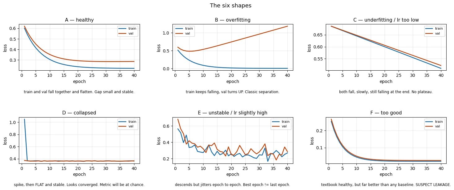
Three of these shapes are especially easy to misread. Commit the reasoning behind them to memory rather than memorising the letters.
D looks like success. A flat, stable loss usually means the optimiser has converged. But convergence only means that the optimisation has stopped making meaningful progress. A model can converge to a useful solution or to a trivial one. The distinguishing evidence is therefore the metric and the prediction distribution, not the fact that the loss is flat.
C looks like a hard problem. A slowly descending curve can tempt you to conclude that the data is weak or the model lacks capacity. But if the curve is still descending when the epoch budget ends, the experiment may simply be undertrained. You have measured how far the optimiser got, not the performance the model would reach if it had enough training.
F looks like a triumph. An unexpectedly excellent result is not automatically evidence that the model is excellent. It can be evidence that the experiment is broken — for example through validation leakage or target leakage. A result that is dramatically better than a sensible baseline should trigger an investigation into why before it triggers celebration.
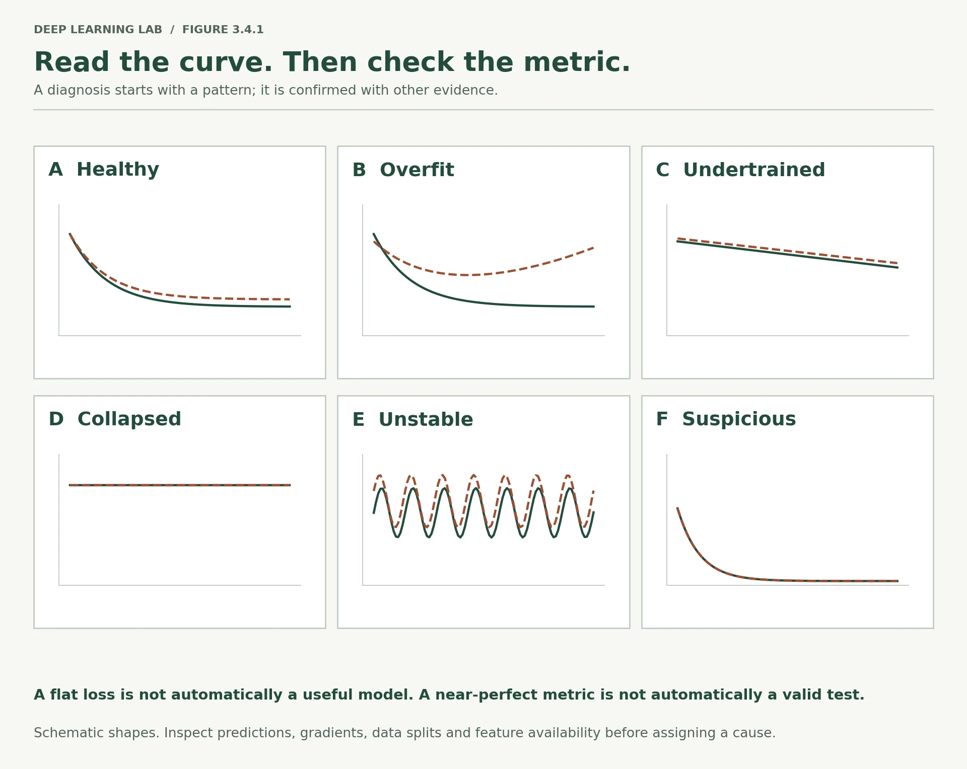
The six shapes above as a memory card: the shape tells you where to look, the metric next to it tells you what happened.
-
Shapes C and D both end with a curve that stops moving. What evidence, other than the loss itself, distinguishes them? Explain why a flat loss is compatible with both healthy convergence and collapse.
Look at what the model does, not at the loss. Shape C's curve is still sloping at the last epoch (measure the slope over the final few epochs), its validation AUC is still rising, and its predictions vary from row to row. Shape D sits flat at about the loss of a constant prediction at the base rate, its AUC is near 0.5, and its predictions are nearly identical for every row; its first epoch also shows a spike. A flat loss only says the optimiser has stopped changing the objective. That happens at a useful minimum and at the trivial constant solution alike, so the value of the plateau (compared with the base-rate loss) and the metric decide which.
-
Shape F is described as dangerous. Why can an apparently excellent result be evidence that you should investigate the experiment rather than trust the model?
Because a result far beyond a sensible baseline is more likely to come from a broken experiment than from a breakthrough. German Credit models are published around 0.78–0.80 AUC; a run at 0.99 is far more often caused by leakage (training rows in validation, a feature that encodes the label, duplicates across the split) than by a better model. Good numbers are also the ones nobody questions, so a bug that produces them survives review. Explain why the result is so good (which features, which split, which rows) before you trust it.
-
You see shape E and the final-epoch score is worse than the best-epoch score. What does that tell you about the relationship between the current checkpoint and the best checkpoint, and what stopping/checkpointing behaviour should you consider?
The last checkpoint is not the best one: the optimiser is bouncing around a good region, and the final epoch landed on a worse point of that noisy trajectory. Keep the best validation checkpoint (early stopping with restore, with patience large enough for the jitter), and consider a smaller learning rate or a decaying schedule (Lesson 3.1 §8) so later epochs settle instead of jumping around. Report that restored checkpoint, and confirm it on the test split.
Shape D is a flat, stable loss. What does 'converged' actually tell you?
Convergence is not success. The metric and the prediction distribution tell you which kind of solution it is.
A result dramatically better than a sensible baseline (shape F) should first trigger…
Excellent numbers can come from a broken experiment. Explain why before you trust it.
Shapes C and D both end with a curve that barely moves. What evidence, other than the loss, tells them apart?
- C (undertrained) is still descending at the end, and the validation metric is still improving; D has plateaued.
- For D, check the metric and predictions: AUC at chance and near-constant predictions mean collapse; good AUC and varied predictions mean healthy convergence.
The harness
Module 2, Lesson 2.4 ended by extracting the notebook into a project repository with a config-driven entry point:
python -m src.training.train --config configs/baseline.yaml
The important idea is that the experiment's settings live in a configuration rather than being scattered through the training code. The runner can therefore execute the same pipeline repeatedly while changing a controlled set of values.
That is exactly what we need here. Six diagnostic cases are only useful if the underlying pipeline stays the same. Otherwise, when a result changes, you cannot tell which change caused it.
This notebook extends the earlier harness in two ways:
- it supports both datasets, selected through a configuration key; and
- it records per-layer gradient norms from Lesson 3.3 alongside the loss and metric history.
A run therefore carries several kinds of evidence:
- loss history — how optimisation progressed;
- validation metrics — whether the model's behaviour is useful on held-out data;
- prediction summaries — whether the model is producing varied, informative outputs;
- gradient profiles — whether different parts of the network are receiving a usable learning signal;
- configuration — exactly what settings produced the run.
This is what makes the later diagnosis reproducible rather than anecdotal.
# ---------------------------------------------------------------- data loadingdef load_bank_marketing(include_duration=False): """Load UCI Bank Marketing, downloading and caching the CSV the first time. Args: include_duration: Keep the ``duration`` column (Case 6's target leak). It is dropped by default because call length is only known after the call. Returns: A tuple ``(X, y)``: the feature DataFrame and a float32 label array (1 = subscribed). """ CSV = "data/bank-full.csv" if not os.path.exists(CSV): url = "https://archive.ics.uci.edu/static/public/222/bank+marketing.zip" raw = urllib.request.urlopen(url, timeout=120).read() outer = zipfile.ZipFile(io.BytesIO(raw)) inner = zipfile.ZipFile(io.BytesIO(outer.read("bank.zip"))) open(CSV, "wb").write(inner.read("bank-full.csv")) df = pd.read_csv(CSV, sep=";") y = (df["y"] == "yes").astype(np.float32).values drop = ["y"] if include_duration else ["y", "duration"] return df.drop(columns=drop), ydef load_german_credit(): """Load German Credit from OpenML (cached locally by scikit-learn). Returns: A tuple ``(X, y)``: the 20-column feature DataFrame and a float32 label array (1 = bad credit risk). """ d = fetch_openml("credit-g", version=1, as_frame=True) return d.data.copy(), (d.target == "bad").astype(np.float32).valuesdef prepare(cfg): """Build training and validation tensors for the dataset a config names. Splits with a fixed seed (German Credit: 500 training rows; Bank Marketing: 80%), halves the remainder into validation and an unused test part, and fits scaling and one-hot encoding on the training rows only. With ``leak_split`` the validation set is replaced by the first training rows, the deliberate bug of Case 4. Args: cfg: Experiment config; reads ``dataset``, ``include_duration`` and ``leak_split``. Returns: A tuple ``(Xt, Yt, Xv, Yv, ytr, yva, d_in)``: training and validation tensors (labels shaped ``(N, 1)``), the NumPy label arrays and the encoded feature count. """ name = cfg.get("dataset", "german_credit") if name == "german_credit": X, y = load_german_credit(); train_size = 500 else: X, y = load_bank_marketing(include_duration=cfg.get("include_duration", False)) train_size = 0.8 num = X.select_dtypes(include="number").columns.tolist() cat = [c for c in X.columns if c not in num] Xtr, Xtmp, ytr, ytmp = train_test_split(X, y, train_size=train_size, random_state=SEED, stratify=y) Xva, _, yva, _ = train_test_split(Xtmp, ytmp, test_size=0.5, random_state=SEED, stratify=ytmp) if cfg.get("leak_split", False): # BUG: validation rows are drawn from the training rows. n = len(Xva) Xva, yva = Xtr.iloc[:n].copy(), ytr[:n].copy() pre = ColumnTransformer([("n", StandardScaler(), num), ("c", OneHotEncoder(handle_unknown="ignore", sparse_output=False), cat)]) A = pre.fit_transform(Xtr).astype(np.float32) V = pre.transform(Xva).astype(np.float32) return (torch.tensor(A), torch.tensor(ytr).unsqueeze(1), torch.tensor(V), torch.tensor(yva).unsqueeze(1), ytr, yva, A.shape[1])- 1
Bank Marketing: 80% train, then the remaining 20% split in half, so validation is 10% of the data (about 4,500 rows).
- 2
The test half is discarded (
_): this clinic only needs training and validation. - 3
The deliberate bug of Case 4: "validation" becomes the first n training rows.
- 4
The preprocessing is fitted on training rows only, as always.
# ------------------------------------------------------------------- the modeldef build_model(cfg, d_in): """Build the MLP a config describes, with an optional non-default initialisation. Args: cfg: Experiment config; reads ``seed``, ``hidden`` (hidden widths), ``dropout``, ``init`` (``"default"``, ``"zeros"`` or ``"big"``) and ``init_std``. d_in: Number of input features. Returns: An ``nn.Sequential`` producing one logit per row. """ torch.manual_seed(cfg.get("seed", SEED)) hidden = tuple(cfg.get("hidden", (64, 32))) p = cfg.get("dropout", 0.0) layers, prev = [], d_in for h in hidden: layers += [nn.Linear(prev, h), nn.ReLU()] if p > 0: layers.append(nn.Dropout(p)) prev = h layers.append(nn.Linear(prev, 1)) model = nn.Sequential(*layers) init = cfg.get("init", "default") if init != "default": for mod in model: if isinstance(mod, nn.Linear): if init == "zeros": nn.init.zeros_(mod.weight); nn.init.zeros_(mod.bias) elif init == "big": nn.init.normal_(mod.weight, 0.0, float(cfg.get("init_std", 3.0))) nn.init.zeros_(mod.bias) return modeldef layer_grad_norms(model, xb, yb): """One forward/backward pass, then the gradient norm of every weight matrix. The Lesson 3.3 probe, returned as a plain dict so it can be saved in the run's JSON. Gradients are cleared before and after. Args: model: The model to probe. xb: A batch of inputs. yb: The matching targets. Returns: A dict mapping each 2-D parameter's name to its gradient norm, in forward order. """ model.train(); model.zero_grad() loss_fn(model(xb), yb).backward() out = {n: p.grad.norm().item() for n, p in model.named_parameters() if p.grad is not None and p.dim() > 1} model.zero_grad() return out# ----------------------------------------------------------------- the runnerdef run_experiment(cfg, save=True, quiet=False): """Run one experiment from a config and return everything it measured. Prepares the data, builds the model, records the gradient profile at initialisation, trains with AdamW (optionally clipping gradients), and after every epoch records losses, AUCs and validation accuracy. The result summarises the final and best scores and the distribution of validation predictions. Args: cfg: Experiment config (``name``, ``dataset``, ``hidden``, ``lr``, ``epochs``, ``batch_size``, ``weight_decay``, ``dropout``, ``init``, ``clip``, ``seed``, ``leak_split``, ``include_duration``); missing keys use the defaults. save: Write the result to ``results/<name>.json``. quiet: Do not print the one-line summary. Returns: A dict with ``config``, ``history`` (one record per epoch), ``grads_at_start``, ``grad_ratio`` (last/first layer), ``final``, ``best_val_loss``, ``best_val_auc``, ``majority_acc``, prediction ``pred_min``/``pred_max``/ ``pred_std``, ``n_unique_preds`` and ``seconds``. """ Xt, Yt, Xv, Yv, ytr, yva, d_in = prepare(cfg) model = build_model(cfg, d_in) opt = torch.optim.AdamW(model.parameters(), lr=cfg.get("lr", 1e-3), weight_decay=cfg.get("weight_decay", 0.0)) g = torch.Generator().manual_seed(cfg.get("seed", SEED)) loader = torch.utils.data.DataLoader( torch.utils.data.TensorDataset(Xt, Yt), batch_size=cfg.get("batch_size", 32), shuffle=True, generator=g) probe_x, probe_y = Xt[:256], Yt[:256] grads_at_start = layer_grad_norms(model, probe_x, probe_y) history, t0 = [], time.time() for ep in range(1, cfg.get("epochs", 40) + 1): model.train() tot = n = 0 for xb, yb in loader: opt.zero_grad(); l = loss_fn(model(xb), yb); l.backward() if cfg.get("clip"): nn.utils.clip_grad_norm_(model.parameters(), cfg["clip"]) opt.step(); tot += l.item()*len(xb); n += len(xb) model.eval() with torch.no_grad(): a, b = model(Xt), model(Xv) pa = torch.sigmoid(a).numpy().ravel(); pb = torch.sigmoid(b).numpy().ravel() history.append(dict( epoch=ep, train_loss=tot/n, val_loss=loss_fn(b, Yv).item(), train_auc=float(roc_auc_score(ytr, pa)), val_auc=float(roc_auc_score(yva, pb)), val_acc=float(accuracy_score(yva, pb > 0.5)))) model.eval() with torch.no_grad(): pb = torch.sigmoid(model(Xv)).numpy().ravel() result = dict( config=cfg, history=history, grads_at_start=grads_at_start, grad_ratio=(list(grads_at_start.values())[-1] / max(list(grads_at_start.values())[0], 1e-30)), final=history[-1], best_val_loss=min(h["val_loss"] for h in history), best_val_auc=max(h["val_auc"] for h in history), majority_acc=float(max(yva.mean(), 1-yva.mean())), pred_min=float(pb.min()), pred_max=float(pb.max()), pred_std=float(pb.std()), n_unique_preds=int(len(np.unique(pb.round(4)))), seconds=time.time()-t0) if save: with open(f"results/{cfg.get('name','run')}.json", "w") as f: json.dump(result, f, indent=2) if not quiet: print(f"[{cfg.get('name','run')}] {cfg.get('dataset','german_credit')} " f"{result['seconds']:.1f}s final val AUC {result['final']['val_auc']:.4f} " f"best val AUC {result['best_val_auc']:.4f}") return resultdef show(result, title=None): """Plot a run: loss curves, AUC curves and the gradient profile at initialisation. Args: result: A result dict from ``run_experiment``. title: Figure title; defaults to the config's name. """ h = result["history"]; e = [x["epoch"] for x in h] fig, axes = plt.subplots(1, 3, figsize=(15, 3.8)) axes[0].plot(e, [x["train_loss"] for x in h], label="train", color="#1b6ca8", lw=1.8) axes[0].plot(e, [x["val_loss"] for x in h], label="val", color="#c1440e", lw=1.8) axes[0].set_ylabel("loss"); axes[0].set_title("loss") axes[1].plot(e, [x["train_auc"] for x in h], label="train", color="#1b6ca8", lw=1.8) axes[1].plot(e, [x["val_auc"] for x in h], label="val", color="#c1440e", lw=1.8) axes[1].axhline(0.5, ls=":", c="0.4", lw=1); axes[1].set_ylabel("ROC-AUC"); axes[1].set_title("AUC") gn = list(result["grads_at_start"].values()) axes[2].plot(range(1, len(gn)+1), gn, "o-", color="#2e7d32", lw=1.8) axes[2].set_yscale("log"); axes[2].set_xlabel("layer"); axes[2].set_ylabel("grad norm") axes[2].set_title("gradient profile at init") for a in axes[:2]: a.set_xlabel("epoch"); a.legend(fontsize=8) for a in axes: a.grid(alpha=0.3) plt.suptitle(title or result["config"].get("name",""), y=1.03) plt.tight_layout(); plt.show()BASELINE = dict(name="baseline", dataset="german_credit", hidden=(64,32), lr=1e-3, epochs=40, batch_size=32)ref = run_experiment(BASELINE)show(ref, "REFERENCE — what correct looks like on German Credit")Everything about a run comes from cfg, and everything it measured goes into one JSON-serialisable result.
- 1
Measured before training: the profile of the freshly initialised network.
- 2
Optional gradient clipping, in the right place: after
backward, beforestep. - 3
Last layer's gradient norm over the first layer's: large means vanishing on the way down.
- 4
Distinct predictions to four decimals: 1 or 2 means collapse, a handful means saturation.
- 5
Every run leaves a record on disk, which can be re-plotted or compared later without retraining.
[baseline] german_credit 0.7s final val AUC 0.7245 best val AUC 0.8158
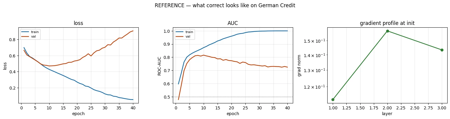
That is the reference run: the example of what normal behaviour looks like when the same pipeline is configured sensibly.
Every case below changes one key in the configuration unless the section explicitly says otherwise. Keep the reference numbers visible while you work. The reference has a final validation AUC around 0.74 and a best validation AUC around 0.82, on a dataset where majority-class accuracy is 0.70 and published results are reported around 0.78–0.80 AUC.
These values are not universal targets. They are a local reference for this exact dataset, split, preprocessing pipeline, model family, and evaluation setup.
That is what a baseline is for. Diagnosis is fundamentally comparative: you cannot call a run abnormal unless you know what normal looks like under the same experimental conditions.
A useful mental model is:
Baseline = your control condition.
If the baseline changes every time you diagnose a problem, you lose the ability to attribute differences to the suspected fault.
Why does every case change only one configuration key from the baseline?
Diagnosis is comparative: you cannot call a run abnormal unless you know what normal looks like under the same conditions.
A diagnostic protocol
When a training run looks wrong, the tempting response is to change something plausible and run it again. That is search, not diagnosis.
Search can eventually find a working configuration, but it does not necessarily tell you why the original run failed. It is also expensive: every retraining attempt consumes time and introduces another result that must be interpreted.
The protocol below is therefore ordered by cost, not by how interesting a test feels.
The protocol, one tier at a time
1. Tier 0: read what the run already gave you (free)
- Are the losses finite? 2. Is the metric above chance, and accuracy above the majority rate? 3. What do the predictions look like: range, spread, number of distinct values? 4. Is the result implausibly better than a sensible baseline?
Rules out or flags: NaNs, collapse to a constant, over-regularisation, and "too good to be true" results (leakage).
2. Tier 1: look inside the model (no retraining)
- Total gradient norm. 6. The per-layer gradient profile. 7. The fraction of dead ReLU units.
Rules out or flags: exploding and vanishing gradients, dead layers, a bad initialisation.
3. Tier 2: run something (costs a training cycle)
- Can the model memorise 20 rows? 9. A learning-rate sweep across orders of magnitude. 10. Regularisation or capacity changes, only when the evidence points there.
Rules out or flags: structural bugs in model, data or loss (if 20 rows can't be memorised), and learning-rate problems.
4. Then: one change, and check the prediction
State the diagnosis, make the smallest change that tests it, and check the result moves the way your hypothesis predicted. If it does not, the diagnosis was wrong, which is also information.
Tier 0 — free checks, before retraining
These use information already produced by the run.
-
Are the losses finite?
If the loss isNaNorInf, downstream metrics and comparisons cannot be trusted. -
What is the metric doing?
A stable loss with AUC near chance can indicate that the model has converged to a useless solution rather than a useful one. -
What do the predictions look like?
Inspect their minimum, maximum, spread, and number of distinct values. A model producing essentially one value has collapsed. A model producing only a narrow band of probabilities may be heavily regularised or otherwise unable to separate decisions. -
Is the result implausibly better than a sensible baseline?
If yes, investigate leakage before interpreting the number as genuine model quality.
Tier 1 — one forward/backward pass
These require looking inside the model, but do not require a full retraining run.
-
Total gradient norm.
Extremely large gradients suggest explosion; extremely small gradients can indicate that the learning signal has disappeared. -
Per-layer gradient profile.
Compare gradient magnitudes across layers. If one part of a network receives much less signal than another, the network may not be training uniformly. -
Dead-unit fraction.
For ReLU networks, inspect how many units are persistently inactive.
Tier 2 — checks that require another run
-
Can the model overfit a tiny subset?
Take 20 rows and deliberately train until the loss is near zero. A model that cannot memorise a tiny, fixed dataset has a structural problem somewhere in the model, data pipeline, or loss. This is one of the highest-value debugging tests because it sharply narrows the search. -
Learning-rate sweep.
Test learning rates across orders of magnitude rather than nudging the value blindly. -
Regularisation and capacity changes.
Only after the earlier evidence points in this direction should you change dropout, weight decay, width, depth, or related capacity controls.
The ordering is deliberate. The expensive checks are often the ones that feel most productive, but the cheap checks can eliminate whole classes of explanations before you spend another training cycle.
What each tier costs, and what it can rule out
Seconds. Rules out NaN, collapse (one prediction), threshold failures (accuracy = majority) and too-good-to-be-true results.
A second or two. Rules out exploding or vanishing gradients and mass-dead ReLUs.
Minutes to days. Tests hypotheses: can it memorise 20 rows? does another learning rate or less regularisation fix it?
def tier0(result, name=""): """Print the Tier 0 checks for a finished run: no retraining needed. Shows the final losses and whether they are finite, final and best validation AUC, accuracy against the majority-class rate, the range, spread and number of distinct predictions, and the gradient ratio at initialisation. Args: result: A result dict from ``run_experiment``. name: Label for the printout. """ f = result["final"] print(f"--- Tier 0: {name} ---") print(f" final train loss / val loss : {f['train_loss']:.4f} / {f['val_loss']:.4f}") print(f" finite? : {np.isfinite(f['train_loss']) and np.isfinite(f['val_loss'])}") print(f" final val AUC : {f['val_auc']:.4f} (chance = 0.5000)") print(f" best val AUC : {result['best_val_auc']:.4f}") print(f" final val accuracy : {f['val_acc']:.4f} (majority = {result['majority_acc']:.4f})") print(f" predictions: min {result['pred_min']:.4f} max {result['pred_max']:.4f} " f"std {result['pred_std']:.3e} distinct {result['n_unique_preds']}") print(f" grad ratio last/first : {result['grad_ratio']:.3e}")def overfit_tiny(cfg, n=20, epochs=200): """Tier 2 check: can this setup memorise a handful of training rows? Trains a fresh model from the config full-batch on the first ``n`` training rows for ``epochs`` steps and prints PASS if the final loss is below 0.05. Args: cfg: Experiment config for the model, data and learning rate. n: Number of training rows to memorise. epochs: Number of full-batch optimizer steps. Returns: The final training loss on those rows. """ Xt, Yt, *_ = prepare(cfg) Xs, Ys = Xt[:n], Yt[:n] model = build_model(cfg, Xt.shape[1]) opt = torch.optim.AdamW(model.parameters(), lr=cfg.get("lr", 1e-3)) for _ in range(epochs): model.train(); opt.zero_grad() loss_fn(model(Xs), Ys).backward(); opt.step() model.eval() with torch.no_grad(): final = loss_fn(model(Xs), Ys).item() verdict = "PASS - setup can learn" if final < 0.05 else "FAIL - bug in model/data/loss" print(f" overfit-{n}-rows check: final loss {final:.5f} -> {verdict}") return finaltier0(ref, "reference")overfit_tiny(BASELINE)- 1
Just 20 training rows.
- 2
Full-batch: the same 20 rows every step, 200 steps. A working setup drives the loss towards zero.
- 3
A loss below 0.05 means the model can memorise; anything above suggests broken wiring.
--- Tier 0: reference ---
  final train loss / val loss : 0.0551 / 0.9040
  finite?                     : True
  final val AUC               : 0.7245   (chance = 0.5000)
  best  val AUC               : 0.8158
  final val accuracy          : 0.7160   (majority = 0.7000)
  predictions: min 0.0000  max 0.9992  std 3.638e-01  distinct 205
  grad ratio last/first       : 1.274e+00
  overfit-20-rows check: final loss 0.00162   -> PASS - setup can learn
0.00162329594604671
The reference run passes the protocol:
- losses remain finite;
- AUC is clearly above chance;
- accuracy is above the majority-class rate;
- predictions span a wide range and contain hundreds of distinct values;
- the gradient profile is reasonably flat across layers; and
- the model can memorise 20 rows when explicitly asked to do so.
That gives us a concrete picture of normal.
The six cases that follow each violate a different part of that picture. Your job is not to spot the answer from the section title. First inspect the evidence, then state the diagnosis, then use the proposed fix to test whether the diagnosis was actually correct.
-
The protocol is ordered by cost rather than by likelihood. Explain how a cheap test can save time even when it does not directly identify the fault.
A test that does not find the fault still eliminates explanations. Finite losses rule out NaN problems; a spread of predictions rules out collapse; AUC above chance rules out a dead model. Each seconds-long negative result shrinks the list of suspects, so the next, more expensive test is aimed at what is left. Ordering by cost also means that when a cheap test does find the fault, you never pay for the expensive ones. Running a retraining experiment first costs minutes or hours even when a free check would have answered the question.
-
The reference predictions span 0.0000 to 0.9992 with 205 distinct values. Which later faults would that single observation make less likely, and why?
A range from 0.0000 to 0.9992 with 205 distinct values over 250 rows rules out anything that makes predictions nearly constant or compressed: collapse (Case 1: 2 distinct values in 0.20–0.35), over-regularisation (Case 3: 0.28–0.42, nothing above 0.5), and a dead or zero-initialised network (one constant value). It also argues against saturation from a bad initialisation, which gives extreme but few distinct values (Case 5: 7). It says nothing about leakage (Cases 4 and 6 have well-spread predictions too): a well-behaved output distribution is not evidence of a valid experiment.
-
overfit_tinyis in Tier 2 rather than Tier 1. What additional cost does it introduce, and what structural question does failure to memorise 20 rows answer that a Tier 0 prediction summary cannot?It costs a new training run: 200 full-batch steps on 20 rows (under a second here, but minutes to hours on a large model), plus code to build the subset. It answers a capability question: can this exact model, data pipeline and loss fit anything when generalisation is taken out of the picture? Failing to memorise 20 rows means the wiring is broken: labels misaligned with inputs, a sigmoid in
forwardfed toBCEWithLogitsLoss, frozen or unregistered parameters, a learning rate orders of magnitude off, a bug in the batch. A Tier 0 summary shows what the trained model outputs; it cannot tell you whether the setup was ever able to learn.
Which check does the protocol run first?
Tier 0 checks are free (finite losses, metric, predictions, baseline plausibility). Expensive retraining comes last.
A model cannot drive its loss towards zero on 20 fixed training rows. What does that suggest?
Any reasonable model should memorise 20 rows. Failing that narrows the search to plumbing, not tuning.
What is the difference between 'search' and 'diagnosis', and why does the protocol order checks by cost?
- Search changes plausible settings and reruns until something works; diagnosis gathers evidence, forms a hypothesis and tests it, so you learn why it failed.
- Cheap checks first can rule out whole classes of explanations before you spend another training run.
Case 1 — learning rate too high
Each case uses the same diagnostic structure:
- inspect the evidence;
- state the most likely diagnosis;
- explain the mechanism that connects the evidence to the diagnosis;
- change the configuration in the smallest defensible way;
- verify that the result improves.
Before reading the diagnosis below the output, pause and make your own statement of the evidence. The important skill is not guessing the answer; it is being able to justify it.
Case 1 raises the learning rate from 1e-3 to 0.5. Before running it: what will its final validation AUC be? (The reference reaches 0.72 final, 0.82 best.)
0.5029. Nothing crashes and the loss looks calm, but the model has collapsed to almost one prediction. The loss settles at 0.6158, right next to the 0.6109 of a constant base-rate prediction.
case1 = run_experiment({**BASELINE, "name": "case1", "lr": 0.5})show(case1, "CASE 1")tier0(case1, "case 1")[case1] german_credit 0.6s final val AUC 0.5029 best val AUC 0.5134
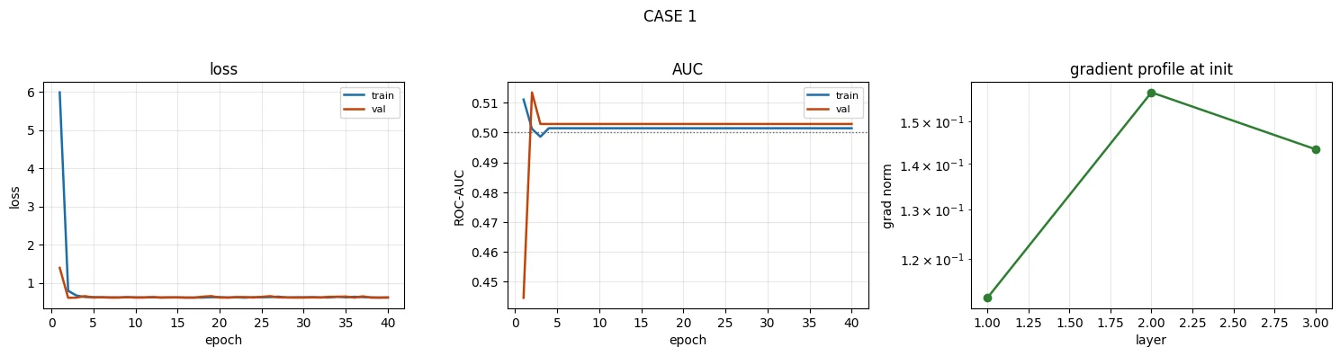
--- Tier 0: case 1 ---
  final train loss / val loss : 0.6116 / 0.6158
  finite?                     : True
  final val AUC               : 0.5029   (chance = 0.5000)
  best  val AUC               : 0.5134
  final val accuracy          : 0.7000   (majority = 0.7000)
  predictions: min 0.2018  max 0.3505  std 9.388e-03  distinct 2
  grad ratio last/first       : 1.274e+00
Evidence. This is gallery shape D: the loss settles into a flat, stable line. The final loss is 0.6158, close to 0.6109, the loss obtained by a constant prediction at the dataset base rate. That is a crucial clue: the loss has not merely stopped improving; it has settled near the loss of the trivial constant predictor.
The validation AUC is at chance, validation accuracy equals the majority-class rate, and the prediction summary is decisive: only two distinct values occur across 250 validation rows, in a narrow range, with a standard deviation far smaller than the reference run.
This is worth distinguishing from the more extreme collapse shown in Lesson 3.1 §6, where every prediction became literally identical. Collapse is a continuum. A model can retain a tiny amount of variation while still having lost almost all useful predictive behaviour.
Diagnosis. The model has collapsed to an almost-constant predictor. The learning rate is too large, so the parameter updates are too aggressive. As discussed in Lesson 3.3, a sufficiently large update can push many first-layer ReLU units into inactive regions. Once those units stop receiving useful gradients, the network can become effectively unable to recover during the run.
Why the loss misleads. Binary cross-entropy has a simple trivial solution: if the model knows only the overall positive rate, predicting that rate for everyone minimises the loss among constant predictions. Therefore a collapsed classifier can have a smooth, stable, apparently "converged" loss.
The important distinction is:
convergence means the optimisation has stopped changing the solution; it does not mean the solution is useful.
That is why the metric and prediction distribution are more informative here than the flat loss curve.
Fix. Reduce the learning rate and retrain from the beginning. Once the network has collapsed, simply changing the learning rate after the fact does not undo the parameter trajectory or restore units that have become inactive.
fix1 = run_experiment({**BASELINE, "name": "case1_fixed", "lr": 1e-3})print(f"\n before: val AUC {case1['final']['val_auc']:.4f}, " f"{case1['n_unique_preds']} distinct predictions")print(f" after : val AUC {fix1['final']['val_auc']:.4f}, " f"{fix1['n_unique_preds']} distinct predictions")[case1_fixed] german_credit 0.6s final val AUC 0.7245 best val AUC 0.8158 before: val AUC 0.5029, 2 distinct predictions after : val AUC 0.7245, 205 distinct predictions
-
Case 1's final validation loss is 0.6158, while a constant prediction at the base rate scores 0.6109. What does that near-match tell you? Why does it make the loss the least informative part of the Tier 0 evidence in this case?
0.6109 is the loss of predicting the base rate, 30% bad, for everyone. Landing at 0.6158 means the model's predictions carry almost no information beyond that base rate: it has learned the class balance and nothing else. That is why the loss is the least informative piece of evidence here: on its own, 0.6158 is a finite, stable, unremarkable number (the reference itself started near 0.70). It only becomes a clue once you compare it with the base-rate loss, while AUC at chance and two distinct predictions show the collapse directly.
-
Only two distinct predictions appear across 250 validation rows, spanning 0.2018 to 0.3505. Why is such a narrow, near-constant range evidence of collapse rather than evidence that the model is simply "confident"?
Confidence is about predictions being extreme, near 0 or 1, and different for different rows. Here every prediction sits between 0.20 and 0.35, around the 0.30 base rate, with a standard deviation of 0.009 (the reference: 0.36) and only two distinct values to four decimals. The model is giving almost everyone the same score: it is not confident, it is not discriminating. A narrow band around the base rate is the signature of a model that has stopped using the features.
-
The fix requires retraining from scratch. Why cannot lowering the learning rate after the collapse simply recover the useful learning trajectory?
Because the damage is in the parameters, not in the learning rate. The oversized updates pushed most first-layer ReLU units into permanently negative territory (60.9% dead at lr = 0.5 in Lesson 3.3). A dead unit receives a zero gradient, and zero times any learning rate is still zero, so a smaller rate cannot move it. The surviving weights have also been thrown far from any useful solution, and Adam's running averages are full of the huge early gradients. Lowering the rate only slows movement from that bad point; it does not rewind to the good trajectory. Start again from a fresh initialisation with the lower rate.
Case 1's loss is 0.6158; a constant base-rate prediction scores 0.6109. What does that near-match tell you?
Two distinct predictions across 250 rows, AUC at chance. The loss is smooth precisely because the trivial solution is stable.
Why can't you rescue the collapsed Case 1 run by lowering the learning rate part-way through?
- The large updates pushed many ReLU units into their zero region; dead units receive no gradient, so lowering the step size gives them nothing to recover with.
- The fix is to restart training from scratch with a sensible learning rate (e.g. 1e-3).
Case 2 — learning rate too low
This case demonstrates the opposite problem.
A learning rate is the scale factor that controls how far the optimiser moves the parameters in response to the gradient. If it is too large, updates can overshoot or destabilise training. If it is too small, training may remain perfectly stable while making too little progress within the available epoch budget.
That second failure is easy to miss because almost everything looks "healthy."
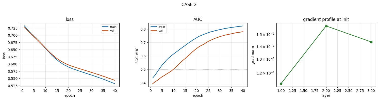
case2 = run_experiment({**BASELINE, "name": "case2", "lr": 1e-4})show(case2, "CASE 2")tier0(case2, "case 2")[case2] german_credit 0.6s final val AUC 0.7803 best val AUC 0.7803
--- Tier 0: case 2 ---
  final train loss / val loss : 0.5316 / 0.5432
  finite?                     : True
  final val AUC               : 0.7803   (chance = 0.5000)
  best  val AUC               : 0.7803
  final val accuracy          : 0.7040   (majority = 0.7000)
  predictions: min 0.1096  max 0.5472  std 8.250e-02  distinct 239
  grad ratio last/first       : 1.274e+00
Evidence. This is gallery shape C. Training and validation loss both descend smoothly, but they are still descending at epoch 40. There is no convincing plateau. Validation AUC is also still climbing: the model is improving, not merely fluctuating around a finished solution. The gradient profile is healthy.
Diagnosis. The run is undertrained. The learning rate is so small that each update moves the parameters only a little. The optimiser therefore needs more epochs than the experiment allows to reach the region that a better learning rate can reach within the same budget.
Why this one is dangerous. There is no dramatic symptom. There is no NaN, explosion, collapse, or obvious instability. If you stop at epoch 40 and report the resulting AUC as the model's capability, you may incorrectly blame the dataset or model class for a result that was caused by the training schedule.
This is the distinction to remember:
A run that has not plateaued has not yet measured its attainable performance.
A low final score is not automatically evidence that the task is hard. First establish whether optimisation has actually finished.
Fix. Raise the learning rate, or use the learning-rate range test from Lesson 3.1 §7 to identify a useful scale directly. Increasing the epoch budget could also allow progress, but if the learning rate is orders of magnitude too small, choosing a sensible learning rate is the more direct test of the diagnosis.
fix2 = run_experiment({**BASELINE, "name": "case2_fixed", "lr": 1e-3})h2, h2f = case2["history"], fix2["history"]print(f"\n broken (lr=1e-4): val AUC {h2[9]['val_auc']:.4f} (ep10) -> {h2[-1]['val_auc']:.4f} (ep40)")print(f" still rising at the end -> the run was cut short, not maxed out")print(f" fixed (lr=1e-3): val AUC {h2f[9]['val_auc']:.4f} (ep10) -> {h2f[-1]['val_auc']:.4f} (ep40)")print(f" reached its peak by epoch 10 and then overfits (see Note 3.2)")[case2_fixed] german_credit 0.6s final val AUC 0.7245 best val AUC 0.8158
broken (lr=1e-4): val AUC 0.5013 (ep10) -> 0.7803 (ep40)
still rising at the end -> the run was cut short, not maxed out
fixed (lr=1e-3): val AUC 0.8158 (ep10) -> 0.7245 (ep40)
reached its peak by epoch 10 and then overfits (see Note 3.2)
-
Case 2's validation AUC is 0.7803, well above chance and not far below the reference's best of 0.8158. What evidence says "undertrained" rather than "this is approximately the best the dataset allows"?
The trajectory, not the level. Validation AUC was still climbing steeply (0.50 at epoch 10, 0.78 at epoch 40) and was at its best on the last epoch; both losses were still falling with no plateau; the training loss (0.53) is nowhere near what the same model reaches at lr = 1e-3 (0.055), so it has not even fitted the training data; and the tiny train/validation gap shows capacity is far from used. Finally, the same architecture reached 0.816 by epoch 10 with a larger learning rate: the dataset clearly allows more.
-
Its final and best validation AUC are the same number. Why is that consistent with an unfinished run, and how does it relate to gallery shape C?
In a finished run the best epoch usually comes before the last: once the model has reached its peak, noise or overfitting pull the final value down. Best = final means the metric was still at its highest when the budget ran out, i.e. still rising. The run was stopped mid-climb, which is exactly gallery shape C: still descending at the end, no plateau, so the attainable performance has not been measured.
-
Name one change other than increasing the learning rate that could improve this run, and explain why it is a less direct diagnostic test of the suspected cause.
Train for many more epochs (say, ten times as many). It would probably improve the run, but it is a weaker test: it costs ten times the compute, and a positive result cannot tell "the step size was too small" apart from "the budget was too short", since for plain undertraining those are the same thing. Raising the learning rate tests the specific hypothesis within the same budget and fails fast if it is wrong. (An LR range test is cheaper still.)
Validation AUC is still rising at the last epoch and final AUC equals best AUC. What should you conclude?
Shape C. Raise the learning rate (or use a range test) before blaming the data or model class.
Case 3 — over-regularised
Regularisation deliberately makes a model less free to fit the training data. Techniques such as dropout, weight decay, and reducing model capacity can improve generalisation when a model is overfitting.
But regularisation has a cost: if it is too strong, it can prevent the model from learning a sufficiently useful function at all.
This case is particularly important because the loss curve itself looks healthy.
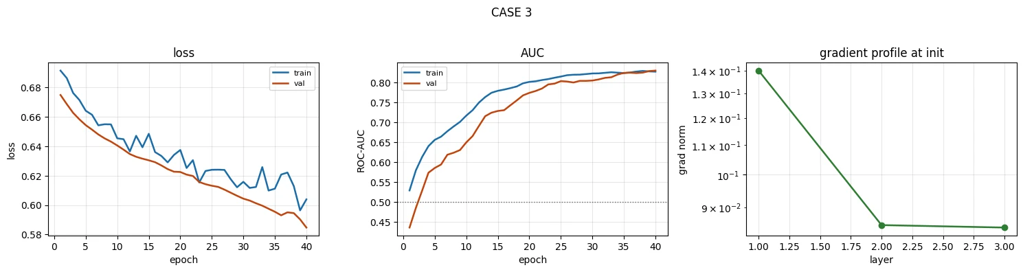
case3 = run_experiment({**BASELINE, "name": "case3", "hidden": (16, 8), "dropout": 0.8, "weight_decay": 1.0})show(case3, "CASE 3")tier0(case3, "case 3")[case3] german_credit 0.6s final val AUC 0.8295 best val AUC 0.8295
--- Tier 0: case 3 ---
  final train loss / val loss : 0.6039 / 0.5847
  finite?                     : True
  final val AUC               : 0.8295   (chance = 0.5000)
  best  val AUC               : 0.8295
  final val accuracy          : 0.7000   (majority = 0.7000)
  predictions: min 0.2769  max 0.4165  std 3.330e-02  distinct 220
  grad ratio last/first       : 6.020e-01
Evidence. The loss curves are calm and well behaved. Validation AUC is respectable, but validation accuracy is exactly the majority-class rate. Predictions are also concentrated in a narrow middle range and do not cross 0.5.
Diagnosis. The model is over-regularised. The small architecture, aggressive dropout, and strong weight decay collectively restrict the model so much that it can retain some ability to rank examples without producing sufficiently separated probabilities for threshold-based decisions.
To understand this, separate two ideas:
- Ranking: are positive examples generally assigned higher scores than negative examples? AUC measures this.
- Classification at a threshold: after choosing a threshold such as 0.5, how many examples are labelled positive or negative? Accuracy depends on this decision rule.
AUC is therefore threshold-free. A model can rank examples reasonably well while leaving every probability below the chosen classification threshold. In that situation, AUC can look good while threshold-based accuracy remains at the majority-class baseline.
The trap. Looking only at AUC would make this model appear successful. Looking only at the loss would also miss the problem. The useful diagnosis comes from combining AUC + accuracy + prediction range.
How to catch it. If AUC is respectable but accuracy equals the majority-class rate and the predictions are tightly clustered, investigate whether regularisation or capacity is preventing the model from separating the classes strongly enough.
Fix. Reduce the regularisation. As Lesson 3.2 established, first make sure early stopping/checkpoint selection is sensible, then add regularisation only when it measurably improves the relevant validation behaviour.
fix3 = run_experiment({**BASELINE, "name": "case3_fixed", "hidden": (16, 8), "dropout": 0.2})print(f"\n over-regularised: val AUC {case3['best_val_auc']:.4f} " f"acc {case3['final']['val_acc']:.4f} pred range [{case3['pred_min']:.3f}, {case3['pred_max']:.3f}]")print(f" fixed : val AUC {fix3['best_val_auc']:.4f} " f"acc {fix3['final']['val_acc']:.4f} pred range [{fix3['pred_min']:.3f}, {fix3['pred_max']:.3f}]")print(f" majority-class accuracy: {case3['majority_acc']:.4f}")[case3_fixed] german_credit 0.6s final val AUC 0.8093 best val AUC 0.8247 over-regularised: val AUC 0.8295 acc 0.7000 pred range [0.277, 0.417] fixed : val AUC 0.8247 acc 0.7360 pred range [0.001, 0.827] majority-class accuracy: 0.7000
-
Case 3 has the highest validation AUC in this notebook, 0.8295, above the reference's 0.8158. Why does that number alone fail to establish that the model is useful?
AUC only measures ranking. This model ranks reasonably, but every predicted probability sits between 0.28 and 0.42, so at the usual 0.5 threshold it flags no one as bad: as a decision-maker it does nothing. Its training loss (0.604) is barely below the 0.611 of a constant prediction, so it has hardly learned to separate the classes at all. And the 0.8295 against 0.8158 gap is well inside the noise floor of a 250-row validation set (Lesson 3.2), so "the highest AUC in the notebook" is not even a reliable ranking.
-
Validation accuracy is 0.7000 and the majority-class rate is 0.7000. What does that imply about the thresholded predictions on this validation set?
That the model predicts "good" for every validation row. Exactly 70% of the rows are good, so labelling everyone good scores exactly 70%, and no prediction exceeds 0.5 (the maximum is 0.4165). At this threshold the model catches none of the 75 bad-credit applicants: recall for the class that matters is zero.
-
Name two additional measurements that reveal the problem that AUC misses. For each, state what pattern you would expect from a healthy model.
Prediction range and spread: a healthy model spreads its predictions widely, on both sides of the threshold (the reference spans 0.0000–0.9992 with a standard deviation of 0.36); here they are squeezed into 0.28–0.42.
Confusion matrix at the operating threshold (or recall and precision for the bad class): a healthy model flags a reasonable number of bad applicants with recall well above zero; here nothing is flagged.
A calibration plot (predicted probability against the observed bad rate in bins) is a good third: healthy is close to the diagonal, over-regularised is a nearly flat line in the middle.
AUC 0.83, accuracy exactly the majority rate, and every prediction between 0.28 and 0.42. Diagnosis?
It ranks reasonably but never crosses 0.5, so it never predicts the positive class. You need AUC + accuracy + prediction range together.
Which two measurements reveal Case 3's problem that AUC misses, and what would a healthy model show on each?
- Thresholded accuracy (or precision/recall): a healthy model beats the majority-class rate; this one equals it.
- Prediction range/spread: a healthy model's predictions spread widely and cross 0.5; these sit in a narrow band (0.28–0.42).
Case 4 — broken validation
The first three cases were failures of the model or training configuration. This case is different: the model may be behaving exactly as instructed, but the experiment has invalid evaluation data.
That distinction is fundamental.
A model is evaluated by comparing its predictions with outcomes on data that represents the situation in which the model will be used. If information from the training set leaks into validation, the validation score no longer estimates performance on genuinely unseen data.
The result can look excellent precisely because the evaluation has stopped being independent.
Case 4 draws its validation rows from the training rows. Its validation AUC will be…
1.0000, with validation tracking training exactly. A beautiful number is the most dangerous kind of broken result, because nobody goes looking for the bug.
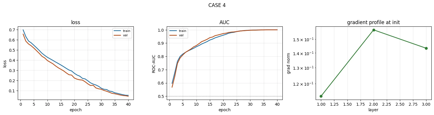
case4 = run_experiment({**BASELINE, "name": "case4", "leak_split": True})show(case4, "CASE 4")tier0(case4, "case 4")print()print(f" reference val AUC : {ref['final']['val_auc']:.4f}")print(f" case 4 val AUC : {case4['final']['val_auc']:.4f}")print(f" train AUC : {case4['final']['train_auc']:.4f}")print(f" val AUC - train AUC gap: {case4['final']['val_auc'] - case4['final']['train_auc']:+.4f}")[case4] german_credit 0.6s final val AUC 1.0000 best val AUC 1.0000
--- Tier 0: case 4 ---
  final train loss / val loss : 0.0551 / 0.0464
  finite?                     : True
  final val AUC               : 1.0000   (chance = 0.5000)
  best  val AUC               : 1.0000
  final val accuracy          : 1.0000   (majority = 0.7200)
  predictions: min 0.0000  max 1.0000  std 4.109e-01  distinct 190
  grad ratio last/first       : 1.274e+00

  reference val AUC : 0.7245
  case 4   val AUC  : 1.0000
  train AUC         : 1.0000
  val AUC - train AUC gap: +0.0000
Evidence. The validation curve tracks the training curve almost exactly. There is effectively no generalisation gap. On the 500-row dataset used here, that is suspicious because the model can reach a training AUC of 1.0 while a genuinely unseen validation set should not simply reproduce the same behaviour.
The validation AUC is also far above the reference run.
Diagnosis. The validation rows are drawn from the training rows. The model is therefore being evaluated on examples it has already seen during training. The label "validation" does not make those rows independent.
This is validation leakage: information that should be held out for evaluation has become available to the training process.
Why this is especially dangerous. Cases 1–3 produce poor or limited numbers, which naturally invite investigation. A broken validation split can produce a beautiful number. That makes the bug more likely to survive review and reach deployment.
More realistic forms of validation leakage
The exact bug here is blatant, but real projects often leak information in subtler ways:
- duplicate records are removed only after the split, allowing duplicates into both sets;
- rows from the same customer or patient are randomly split, so the same entity appears on both sides;
- time-series rows are randomly split, allowing the model to train on information from the future;
- preprocessing statistics are fitted on the full dataset before splitting.
The last case explains the common pipeline pattern:
pre.fit_transform(X_train)
pre.transform(X_val)
The preprocessing object learns its parameters from training data only. Validation data is transformed using those already-learned parameters.
The tell. A validation score that is suspiciously close to, or even better than, training performance deserves an investigation of the split and data flow. A small generalisation gap can be perfectly normal; the point is not that every small gap is leakage, but that an implausibly perfect evaluation should be explained.
Fix. Rebuild the split so that validation examples are genuinely held out. Where rows have a natural group structure, split by the group rather than by individual row.
-
Validation AUC is exactly 1.0000 and the validation-minus-training gap is +0.0000. Which observation is the stronger diagnostic clue that the split is broken, and why is the combination more informative than either number alone?
The zero gap is the stronger clue. A perfect validation AUC could, in principle, come from a genuinely easy problem or a single strong feature (Case 6 shows a leaked feature can do this with a normal gap). But a model that fits its 500 training rows perfectly should always do somewhat worse on rows it has never seen; validation matching training exactly says these rows are behaving like training rows because they are training rows. Together, "perfect" and "identical to training" leave essentially one explanation: the model is being scored on data it has seen. (The 0.7200 majority rate, instead of the stratified 0.7000, points the same way.)
-
This notebook uses a blunt leak: validation rows are copied from training rows. How would you investigate the subtler case where rows are distinct but several rows belong to the same customer?
Look for the entity, not the row. If there is a customer ID, count how many validation customers also appear in training. If not, build a key from stable identifying fields (for example age, job, marital status and credit history) and look for matches, or find each validation row's nearest training row and inspect the suspiciously close pairs. Then compare the score on validation rows whose customer appears in training against rows whose customer does not: a large difference is leakage. The fix is a group split (
GroupShuffleSplitorGroupKFold) so each customer lives in exactly one split. -
Suppose the leak were less obvious and the validation-minus-training gap were −0.02 instead of 0.0000. What would you inspect before deciding that the split is sound?
A gap of −0.02 is perfectly normal, so check the data flow rather than the number: exact and near-duplicate rows across the splits (hash every row); entity overlap as in the previous answer; whether the data has a time order that a random split ignores; whether any preprocessing was fitted before the split; and whether any single feature predicts the label almost perfectly on its own (compute each feature's AUC). Finally, see whether a simple baseline such as logistic regression also scores suspiciously high: if it does, the evaluation, not the network, is the thing to explain.
Validation AUC is 1.0000 and validation exactly matches training. The most likely cause?
On 500 rows, a truly unseen set should not reproduce training behaviour exactly. Beautiful numbers survive review, which makes this dangerous.
Which is a subtle form of validation leakage?
The same entity on both sides lets the model recognise it. Split by group, dedupe before splitting, split time series by time, fit preprocessing on training only.
Case 5 — poor initialisation
A neural network does not begin from a neutral state. Its initial parameter values determine the numerical scale of the first forward pass and therefore the scale of the first backward pass.
Good initialisation aims to keep activations and gradients in a useful numerical range. Poor initialisation can put the network into an extreme state before learning has meaningfully begun.
This case makes that visible by deliberately starting with weights that are far too large.
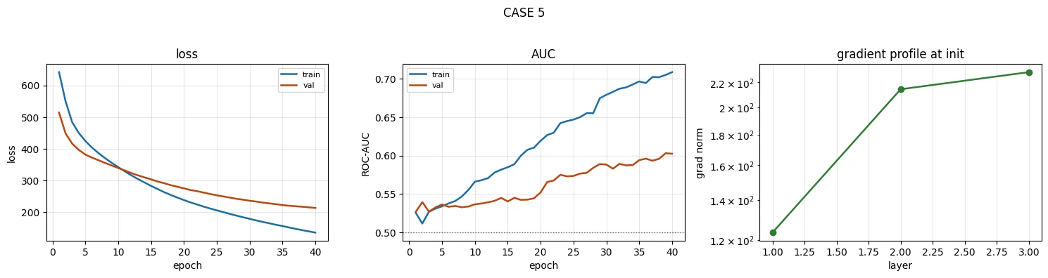
case5 = run_experiment({**BASELINE, "name": "case5", "init": "big", "init_std": 3.0})show(case5, "CASE 5")tier0(case5, "case 5")print()print(" gradient norms at initialisation, per layer:")for k, v in case5["grads_at_start"].items(): print(f" {k:<12} {v:.4e}")print(f" reference, same layers:")for k, v in ref["grads_at_start"].items(): print(f" {k:<12} {v:.4e}")[case5] german_credit 0.6s final val AUC 0.6024 best val AUC 0.6029
--- Tier 0: case 5 ---
  final train loss / val loss : 135.0999 / 212.8671
  finite?                     : True
  final val AUC               : 0.6024   (chance = 0.5000)
  best  val AUC               : 0.6029
  final val accuracy          : 0.6400   (majority = 0.7000)
  predictions: min 0.0000  max 1.0000  std 4.643e-01  distinct 7
  grad ratio last/first       : 1.851e+00

  gradient norms at initialisation, per layer:
    0.weight     1.2359e+02
    2.weight     2.1428e+02
    4.weight     2.2881e+02
  reference, same layers:
    0.weight     1.1257e-01
    2.weight     1.5730e-01
    4.weight     1.4339e-01
Evidence. The first loss is in the hundreds rather than near the roughly 0.6–0.7 range expected for a sensibly initialised binary classifier whose initial predictions are near the dataset base rate. The initial gradient norms are also orders of magnitude larger than those in the reference run.
The loss decreases, but never reaches a reasonable region, and AUC remains poor — below both the reference run and the logistic-regression baseline.
Diagnosis. The weights were initialised far too large. As discussed in Lesson 3.3, oversized weights create oversized pre-activations. That pushes the network into an extreme numerical regime and can produce very large gradients and unstable updates. The optimiser then spends the run trying to recover from a poor starting scale.
The Tier 0 tell that costs almost nothing. For a binary classifier whose initial predictions are close to the base rate p, binary cross-entropy should be near the entropy of that base-rate prediction:
-[p·ln(p) + (1-p)·ln(1-p)]
For this dataset that is around 0.6. The exact number is not the point; the diagnostic principle is.
If the first loss is wildly outside a plausible range, investigate initialisation and input scaling before spending time tuning later training behaviour. The first forward pass is a cheap window into whether the model started in a sensible numerical regime.
p = float(ref["history"][0]["train_loss"])base = 0.30 # positive rate in German Creditexpected = -(base*np.log(base) + (1-base)*np.log(1-base))print(f" expected initial loss for base rate {base}: {expected:.4f}")print(f" reference, epoch-1 train loss : {ref['history'][0]['train_loss']:.4f} <- sane")print(f" case 5, epoch-1 train loss : {case5['history'][0]['train_loss']:.4f} <- not sane")print()fix5 = run_experiment({**BASELINE, "name": "case5_fixed", "init": "default"})print(f"\n broken init: val AUC {case5['final']['val_auc']:.4f}")print(f" default init: val AUC {fix5['final']['val_auc']:.4f}")expected initial loss for base rate 0.3: 0.6109 reference, epoch-1 train loss : 0.6975 <- sane case 5, epoch-1 train loss : 641.6535 <- not sane [case5_fixed] german_credit 0.6s final val AUC 0.7245 best val AUC 0.8158 broken init: val AUC 0.6024 default init: val AUC 0.7245
-
The epoch-1 training loss is 641.65 against an expected value around 0.61 for the dataset base rate. Why is the first loss a more useful clue about initialisation than the final loss?
The first loss describes the model before optimisation has had any chance to compensate, and you know what it should be: about 0.61 (the base-rate loss) or 0.69 (predicting 0.5) for a sensibly initialised binary classifier. A value of 641 can only come from the starting state: enormous logits from enormous weights. The final loss mixes the initialisation with 40 epochs of learning rate, overfitting and everything else, so many different causes could explain a bad final number. (Strictly, "epoch-1 loss" averages the first epoch's batches, but those early batches dominate it.)
-
Initial gradient norms are around
1e+02per layer versus roughly1e-01in the reference. Which Lesson 3.3 pathology does this pattern suggest, and why?Exploding gradients (Lesson 3.3 §4): the norms are about a thousand times the reference's in every layer, and the profile is flat (ratio 1.85), so this is not the depth-driven kind of explosion but a scale problem. Weights with standard deviation 3 produce huge pre-activations and logits, hence a huge loss and huge gradients. AdamW normalises its step size, so the run does not turn into NaN, but it spends its whole budget climbing out of that regime.
-
This case produces 7 distinct predictions spanning nearly the full 0–1 range. How does that differ from Case 1's near-constant prediction collapse, and what does that difference tell you about the underlying failure?
Case 5's predictions are extreme: the logits are so large that most sigmoids round to exactly 0.0000 or 1.0000, which is why only seven distinct values survive across the full 0–1 range. The network still distinguishes rows (AUC 0.60, above chance) but is wildly overconfident, hence the validation loss of 213. Case 1's predictions are near-constant around the base rate: the network has stopped distinguishing rows at all (AUC 0.50). Different outputs, different mechanisms: saturation from oversized weights in Case 5, lost capacity (dead units) from oversized updates in Case 1.
Case 5's first training loss was 641 against an expected ~0.61. Why is the first loss such a useful clue?
\(-(p\log p + (1-p)\log(1-p))\) with \(p = 0.3\) gives ≈ 0.61. Far outside that range points to initialisation or input scaling.
Case 6 — the one that looks fine
Every previous case had an obvious statistical or optimisation symptom.
This one is different.
The curves are healthy. The gradient profile is healthy. The generalisation gap looks normal. Predictions are well spread. The model appears excellent.
And the model is still unusable.
This is the case that forces you to recognise a boundary of model diagnostics: some failures cannot be discovered by looking at the training run alone. You must understand what the features mean and when they exist in the real process.
Case 6 keeps the duration column in Bank Marketing. Validation AUC without it is 0.785. With it?
0.926, and every Tier 0 and Tier 1 check passes. Only the plausibility check fires: +0.14 AUC from one column needs an explanation.
case6 = run_experiment({**BASELINE, "name": "case6", "dataset": "bank_marketing", "include_duration": True, "batch_size": 256, "epochs": 15})show(case6, "CASE 6 — every diagnostic passes")tier0(case6, "case 6")print()clean = run_experiment({**BASELINE, "name": "case6_clean", "dataset": "bank_marketing", "include_duration": False, "batch_size": 256, "epochs": 15})print(f"\n with `duration` : val AUC {case6['final']['val_auc']:.4f}")print(f" without `duration`: val AUC {clean['final']['val_auc']:.4f}")print(f" logistic-regression baseline (Note 3.1): 0.7717")print(f" improvement from one column: {case6['final']['val_auc'] - clean['final']['val_auc']:+.4f} AUC")[case6] bank_marketing 4.3s final val AUC 0.9262 best val AUC 0.9264
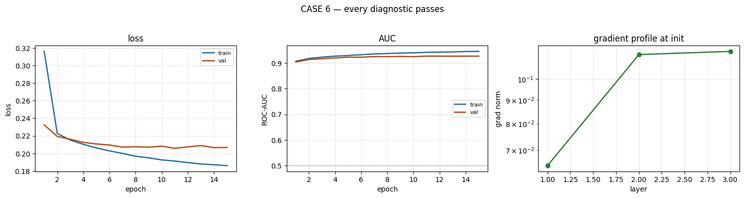
--- Tier 0: case 6 ---
  final train loss / val loss : 0.1860 / 0.2067
  finite?                     : True
  final val AUC               : 0.9262   (chance = 0.5000)
  best  val AUC               : 0.9264
  final val accuracy          : 0.9078   (majority = 0.8830)
  predictions: min 0.0000  max 0.9265  std 2.108e-01  distinct 1681
  grad ratio last/first       : 1.777e+00

[case6_clean] bank_marketing  4.2s   final val AUC 0.7853   best val AUC 0.7853

  with `duration`   : val AUC 0.9262
  without `duration`: val AUC 0.7853
  logistic-regression baseline (Note 3.1): 0.7717
  improvement from one column: +0.1409 AUC
Evidence. There is no obvious internal failure. Every Tier 0 and Tier 1 diagnostic passes. The curves match gallery shape A, gradients are well behaved, predictions are well spread, and the generalisation gap is small and stable.
The only statistical warning is Tier 0 check 4: the result is much better than a sensible baseline and there is no credible explanation for the size of the improvement.
Diagnosis. The problem is the duration feature. It records how long the sales call lasted. Call duration is strongly related to whether the call ultimately succeeds, so it is highly predictive inside the historical dataset.
But the prediction is supposed to answer a question such as "who should we call?" At the moment that decision must be made, the call has not happened yet. Therefore duration does not exist.
This is target leakage: an input contains information that is available only because the outcome, or a process downstream of the outcome, has already occurred.
That makes this different from validation leakage:
- Validation leakage contaminates the separation between training and evaluation data.
- Target leakage uses an input feature that would not be available at the real prediction time.
Why ordinary statistical diagnostics cannot catch this
Within the historical table, duration is simply a very good predictor. Cross-validation can repeatedly confirm that it is predictive. The problem is not that the statistical relationship is false.
The problem is that the relationship is temporally invalid for deployment.
This means leakage is partly a data-science problem and partly a domain-understanding problem. A person has to know where each feature comes from and when it becomes available.
The three questions that catch it
For every feature, ask:
- At the moment I need to make the prediction, does this value exist yet?
- Could this value have been influenced by the outcome I am trying to predict?
- If I deployed the model tomorrow, could I actually obtain this value in time?
A result that is dramatically better than a sensible baseline should therefore be treated as an investigation trigger, not automatically as a success.
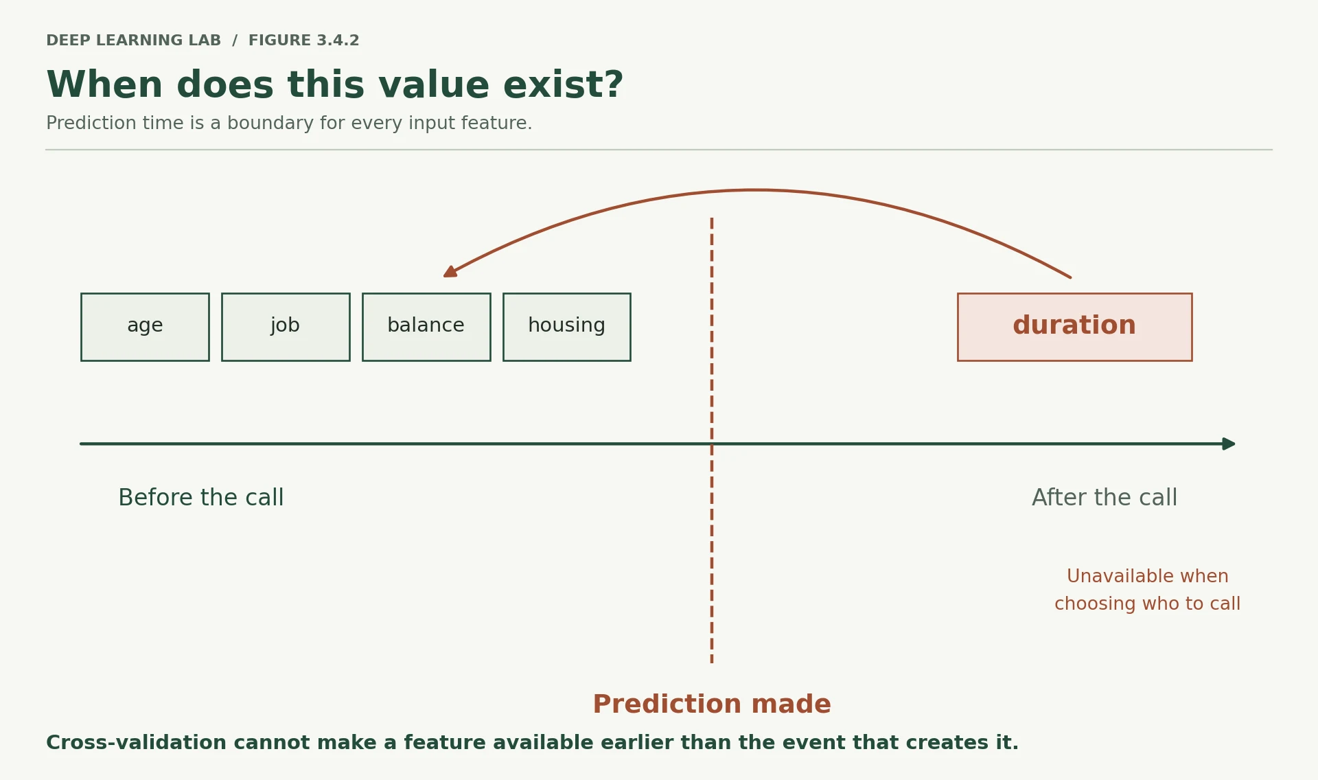
Leakage is a question about time, not about statistics. duration is only known once the call is over, after the decision it is supposed to inform.
-
Every Tier 0 and Tier 1 check passes on Case 6. Which protocol check fires, and what does it compare the result against?
Tier 0 check 4, "is the result implausibly better than a sensible baseline?". It compares 0.926 with the logistic-regression baseline for Bank Marketing (0.7717, Lesson 3.1), with the same network trained without
duration(0.785), and with everything Module 2 achieved (about 0.79–0.80). A single column adding 0.14 AUC, with no domain explanation, is the trigger. -
durationadds about +0.1409 AUC relative to the same model without it. Why would cross-validation still fail to identify this as invalid?Cross-validation only re-splits the same historical table. In every fold, every row still has its
duration, anddurationreally is predictive of the outcome in that table, so every fold confirms it. Cross-validation estimates performance on data collected the same way, and the flaw is that deployment data will not be collected that way: at prediction time the call has not happened. The problem is about when the value exists, and no resampling of a table can see time. -
Apply the three leakage questions to
campaign(number of contacts during this campaign) andpoutcome(outcome of the previous campaign). What information would you need to decide whether either feature is valid at prediction time?campaigncounts contacts during this campaign, and the UCI documentation says it includes the last contact. If you predict before the first call of a campaign, it does not exist yet; if you predict before each new call, a count of calls so far exists, but the stored value may include the very call whose outcome is the label. You need to know when the column was snapshotted relative to the decision.poutcomeis the outcome of the previous campaign, so it is normally known before the current one starts and is likely valid, provided "previous" really means a campaign that finished before this prediction.In both cases: read the data dictionary, find the timestamp at which each value was recorded, and compare it with the moment the prediction must be made.
-
A colleague reports a model that beats your baseline by 0.14 AUC. What are the first two questions you would ask before treating the improvement as genuine?
- Which features does it use, and would every one of them exist at the moment the prediction is made? (target leakage)
- How were training and evaluation data separated (by row, by customer, by time), and could anything cross that boundary? (validation leakage)
Only once both answers are clean is it worth asking whether the model itself is better.
Adding duration raises AUC from 0.785 to 0.926 and every diagnostic passes. Why is the model still unusable?
The statistical relationship is real but temporally invalid for deployment. Cross-validation cannot catch this.
State the three questions to ask of every feature to catch target leakage.
- At the moment I need to make the prediction, does this value exist yet?
- Could this value have been influenced by the outcome I am predicting?
- If I deployed tomorrow, could I actually obtain this value in time?
Your turn
Now the answer key disappears.
There are two configurations below. For each one:
- run the experiment;
- inspect the curve and Tier 0 output;
- work through the protocol from Section 3 in order;
- write the evidence before writing the diagnosis;
- propose the smallest defensible fix;
- run the fix and check whether the result changes in the way your hypothesis predicted.
Resist the urge to guess and immediately re-run. The point of the exercise is to practise evidence → hypothesis → test, not trial-and-error tuning.
A note about Mystery B: it contains more than one fault. That means you will need to distinguish the primary symptoms and avoid stopping after finding the first plausible explanation.
Finish a round of all twelve cases with at least 45 of 60 points.
mystery_a = {**BASELINE, "name": "mystery_a", "hidden": tuple([64]*16), "lr": 1e-3, "epochs": 40}mystery_b = {**BASELINE, "name": "mystery_b", "hidden": (256, 128), "lr": 1e-4, "weight_decay": 2.0, "dropout": 0.6, "epochs": 25}print("Run these, then diagnose. The Tier 0 helper and `show()` are already defined.\n")ma = run_experiment(mystery_a); show(ma, "MYSTERY A"); tier0(ma, "mystery A")Run these, then diagnose. The Tier 0 helper and `show()` are already defined. [mystery_a] german_credit 1.8s final val AUC 0.7073 best val AUC 0.8359
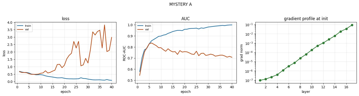
--- Tier 0: mystery A ---
  final train loss / val loss : 0.0828 / 2.9797
  finite?                     : True
  final val AUC               : 0.7073   (chance = 0.5000)
  best  val AUC               : 0.8359
  final val accuracy          : 0.6880   (majority = 0.7000)
  predictions: min 0.0000  max 0.9951  std 3.807e-01  distinct 107
  grad ratio last/first       : 9.466e+05
mb = run_experiment(mystery_b); show(mb, "MYSTERY B"); tier0(mb, "mystery B")[mystery_b] german_credit 0.6s final val AUC 0.8048 best val AUC 0.8048
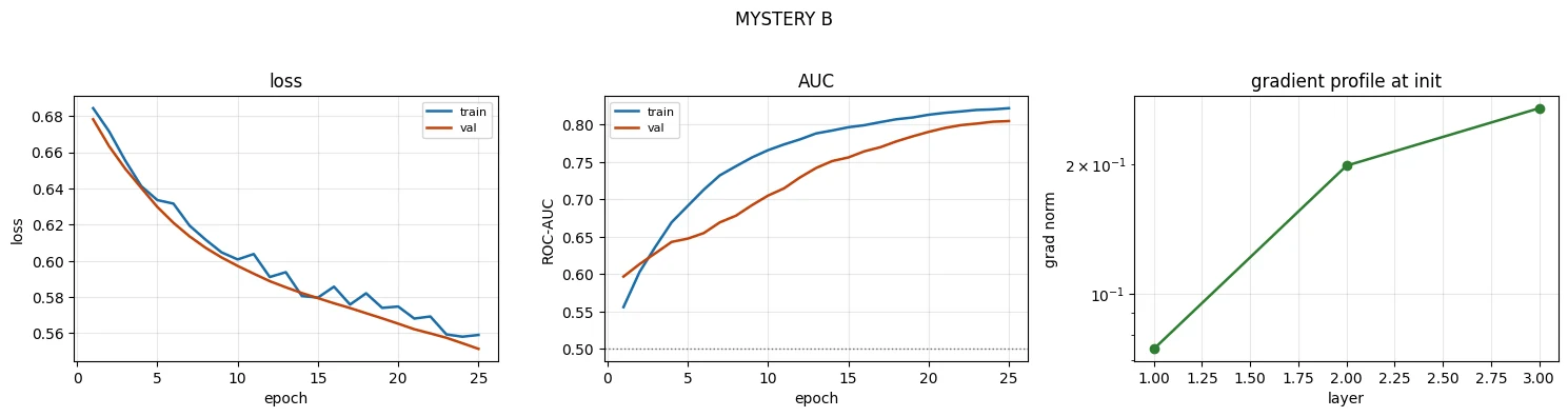
--- Tier 0: mystery B ---
  final train loss / val loss : 0.5591 / 0.5514
  finite?                     : True
  final val AUC               : 0.8048   (chance = 0.5000)
  best  val AUC               : 0.8048
  final val accuracy          : 0.7000   (majority = 0.7000)
  predictions: min 0.1329  max 0.4340  std 6.295e-02  distinct 232
  grad ratio last/first       : 3.634e+00
# Scratch space for your diagnosis.## MYSTERY A# evidence :# diagnosis :# proposed fix:## MYSTERY B# evidence :# diagnosis :# proposed fix:## Test your fixes by editing a copy of the config and re-running, e.g.:# fix_a = run_experiment({**mystery_a, "name": "mystery_a_fixed", "lr": ...})# tier0(fix_a, "mystery A fixed")print("Hints, if you need them:")print(" A — compare the gradient profile panel against the reference run's.")print(" Then count the layers. Then look at what Note 3.3 sections 3, 6 and 7 were about.")print(" B — check the AUC and the accuracy separately, then the prediction range.")print(" Then ask whether the run has plateaued. Two things are wrong, not one.")Hints, if you need them:
A — compare the gradient profile panel against the reference run's.
Then count the layers. Then look at what Note 3.3 sections 3, 6 and 7 were about.
B — check the AUC and the accuracy separately, then the prediction range.
Then ask whether the run has plateaued. Two things are wrong, not one.
Deep diveA worked diagnosis: Mystery A (open after trying it yourself)
Evidence. Tier 0: train loss 0.083 against validation loss 2.98, best validation AUC 0.836 against final 0.707: gallery shape B,
overfitting, and the final checkpoint is far past the best one. Tier 1: gradient ratio last/first 9.5×10⁵, against 1.3 for the
reference. Counting layers: hidden=tuple([64]*16) is 16 hidden layers, 17 weight matrices.
Diagnosis. Two things at once. The plain 17-layer ReLU stack with PyTorch's default initialisation has a vanishing gradient profile (Lesson 3.3): the first layers receive about a millionth of the last layer's signal. That did not stop the model from fitting: the later layers alone have ample capacity to memorise 500 rows, so it also overfits badly once it passes its best epoch.
Smallest fixes to test, one at a time. Depth is the cause of the profile, so first go back to 2 hidden layers (the reference) and confirm the ratio returns to about 1. If depth is required, add normalisation or residual blocks (Lesson 3.3 §6–7), or Kaiming initialisation. Separately, keep the best-epoch checkpoint (early stopping) so overfitting after the peak does not decide the reported number. Note that 0.836 against the reference's 0.816 is inside the noise floor: the deep model is not better.
Deep diveA worked diagnosis: Mystery B (open after trying it yourself)
Evidence. Validation AUC 0.805 looks fine, but accuracy is exactly the majority rate (0.700) and every prediction lies between 0.13 and 0.43: nothing crosses 0.5 (Case 3's signature). Final AUC equals best AUC, so validation was still improving at the last epoch, and the loss is still falling (Case 2's signature). Training loss 0.559 is still close to the 0.611 of a constant prediction.
Diagnosis: two faults. The run is undertrained: lr=1e-4 for only 25 epochs. And it is heavily regularised: dropout 0.6
on top of weight decay 2.0. Be careful attributing the compressed predictions: an undertrained model also stays close to the base
rate, so both faults push in the same direction. And because AdamW's decay per step is lr × weight_decay, 2.0 at lr 1e-4 decays
exactly as fast as 0.2 at lr 1e-3; raise the learning rate and the same setting becomes ten times stronger.
Test them separately. First raise lr to 1e-3 alone: if the prediction range widens and the curve plateaus, undertraining was the
larger fault. Then lower dropout and weight decay with the learning rate fixed, and watch accuracy against the majority rate and the
prediction range. Changing both at once would fix the run and teach you nothing about which fault mattered.
Mystery A uses 16 hidden layers of width 64 and shows a huge train–validation gap. Which lesson's tools should you reach for first?
Deep plain stacks have uneven gradient flow; compare the gradient profile with the reference, then count the layers. Evidence first, then diagnosis.
Writing it up
A diagnosis that cannot be reconstructed three months later is of limited value. The point of an experiment record is not bureaucracy; it is to preserve the reasoning that connects a configuration to an observed result.
The blueprint makes documentation a cross-cutting practice for exactly this reason, and Module 4 will turn it into a formal experiment protocol.
The format below is deliberately minimal. It captures five questions:
- What did I try?
- Why did I try it?
- What happened?
- What did I learn?
- What would I change next?
The log also records the configuration differences from the baseline. That makes the experiment easier to reproduce and makes the causal comparison visible without forcing you to copy a large configuration block every time.
A good record should let your future self reconstruct the reasoning without needing to trust your memory.
def experiment_log(result, hypothesis, diagnosis, action, learned): """Write a short markdown record of an experiment next to its JSON results. The record lists what changed from ``BASELINE``, the hypothesis, the measured result (generated from ``result``), the diagnosis, the action taken and the lesson. Args: result: A result dict from ``run_experiment``. hypothesis: What you expected before running it, and why. diagnosis: Your reading of the evidence. action: What you changed in response. learned: What you would carry into the next experiment. Returns: The path of the markdown file written, ``results/<name>.md``. """ cfg = result["config"]; f = result["final"] changed = {k: v for k, v in cfg.items() if k not in BASELINE or BASELINE.get(k) != v} md_text = f"""### Experiment: {cfg.get('name','run')}**Date/run time:** {result['seconds']:.1f}s on {cfg.get('dataset','german_credit')}**Changed from baseline:** {changed or 'nothing'}**Hypothesis:** {hypothesis}**Result:** final val AUC {f['val_auc']:.4f} (best {result['best_val_auc']:.4f}),val accuracy {f['val_acc']:.4f} against majority {result['majority_acc']:.4f},predictions in [{result['pred_min']:.3f}, {result['pred_max']:.3f}]with {result['n_unique_preds']} distinct values,gradient ratio {result['grad_ratio']:.2e}**Diagnosis:** {diagnosis}**Action taken:** {action}**What I learned:** {learned}""" path = f"results/{cfg.get('name','run')}.md" with open(path, "w") as fh: fh.write(md_text) print(md_text) return pathexperiment_log( case1, hypothesis="A higher learning rate would converge faster than the 1e-3 baseline.", diagnosis=("Collapsed to a constant predictor. Val AUC exactly 0.5000, one distinct " "prediction across the validation set, accuracy equal to the majority rate. " "Loss was flat and stable, which initially looked like convergence."), action="Reverted to lr=1e-3. Confirmed recovery: val AUC returned to the reference level.", learned=("A flat loss is not evidence of convergence. The prediction-spread check in Tier 0 " "identified this in under a second, without retraining."))- 1
Only the keys that differ from
BASELINE(plusname), so the change under test is obvious. - 2
The record sits next to the run's JSON, under the same name.
### Experiment: case1

**Date/run time:** 0.6s on german_credit

**Changed from baseline:** {'name': 'case1', 'lr': 0.5}

**Hypothesis:** A higher learning rate would converge faster than the 1e-3 baseline.

**Result:** final val AUC 0.5029 (best 0.5134),
val accuracy 0.7000 against majority 0.7000,
predictions in [0.202, 0.351]
with 2 distinct values,
gradient ratio 1.27e+00

**Diagnosis:** Collapsed to a constant predictor. Val AUC exactly 0.5000, one distinct prediction across the validation set, accuracy equal to the majority rate. Loss was flat and stable, which initially looked like convergence.

**Action taken:** Reverted to lr=1e-3. Confirmed recovery: val AUC returned to the reference level.

**What I learned:** A flat loss is not evidence of convergence. The prediction-spread check in Tier 0 identified this in under a second, without retraining.
'results/case1.md'
print("files written by this notebook:")for fn in sorted(os.listdir("results")): print(f" results/{fn}")print()print("The JSON files carry the full history and gradient profile for every run,")print("so any of these can be re-plotted or compared later without retraining.")files written by this notebook: results/baseline.json results/case1.json results/case1.md results/case1_fixed.json results/case2.json results/case2_fixed.json results/case3.json results/case3_fixed.json results/case4.json results/case5.json results/case5_fixed.json results/case6.json results/case6_clean.json results/mystery_a.json results/mystery_b.json The JSON files carry the full history and gradient profile for every run, so any of these can be re-plotted or compared later without retraining.
-
The record separates the hypothesis from the diagnosis. Why does writing the hypothesis before the run change what you can learn from the result?
A hypothesis written before the run is a prediction that can fail: comparing it with the result tells you whether your understanding of the system is right. Written afterwards, it tends to be shaped by the result (hindsight), so every outcome looks "expected" and you learn nothing. Writing it first also forces you to decide what evidence would prove you wrong, so you measure the right things.
-
The log stores the configuration keys that differ from the baseline rather than the entire configuration. What does that make easier to read and compare, and what information might you lose?
Easier: you see at a glance what changed, runs can be compared line by line, and a confound (two keys changed at once) jumps out. Lost: anything not in the config. The diff is relative to
BASELINE, which may itself change later; defaults hidden in code (AdamW's betas, the initialisation scheme, the probe batch) do not appear; nor do library versions, the data version or the hardware. The JSON file next to it stores the full configuration, which covers part of this; recording the baseline's version and the package versions covers the rest. -
Choose any case in this notebook and reconstruct its record in four sentences without looking back at the diagnosis text. Which part is hardest to reconstruct? That difficulty is evidence about what you should have written down during the experiment.
For example, Case 2: "Hypothesis: lr = 1e-4 would train more stably than 1e-3. Result: validation AUC 0.780 and still rising at epoch 40, best = final, losses still falling. Diagnosis: undertrained, the step size is too small for the 40-epoch budget. Fix: lr = 1e-3 reaches 0.816 by epoch 10." Most people find the hypothesis hardest: the reason a run was started is rarely visible in its outputs, so it is lost unless it is written down before the run.
What to take away
Diagnose before you intervene. Changing something plausible and re-running is search, not diagnosis. It can find a working configuration while teaching you very little about the original failure.
Order checks by cost. Tier 0 checks — finite losses, metrics, prediction spread, majority-class comparison, and baseline plausibility — cost almost nothing. Use them before spending another training cycle.
The loss is evidence, not the diagnosis. A flat loss can mean healthy convergence or collapse. A smooth descending loss can mean genuine progress or simply that the run has not trained long enough. Always read the loss alongside metrics, predictions, and the reference run.
Use prediction behaviour as a first-class diagnostic. A model that emits nearly one value has a very different problem from a model whose predictions are spread across the full range. The metric alone may not reveal that distinction.
The tiny-subset overfit test is a powerful structural check. If the model cannot memorise a tiny set of examples when deliberately given enough optimisation, suspect the model, data pipeline, or loss before tuning ordinary hyperparameters.
Good numbers deserve scrutiny too. A broken validation split can produce excellent validation scores. A leaked feature can produce excellent curves and healthy gradients. Statistical diagnostics cannot replace knowledge of how the data was generated and when each feature becomes available.
Write the reasoning down while it is fresh. A short experiment record turns a training run into reusable knowledge rather than another result you will have to rediscover later.
Where Module 3 leaves you
You began the day able to write a training loop. You can now:
- choose an optimiser and learning rate with a reason, and identify a sensible learning-rate scale;
- recognise common learning-rate and loss-curve signatures;
- deliberately create overfitting and choose an intervention based on evidence;
- distinguish a genuine improvement from variation by measuring the relevant noise;
- inspect a network's gradient profile layer by layer;
- identify and explain vanishing gradients, exploding gradients, and dead units;
- work from an unfamiliar symptom to a testable diagnosis and then to a defensible intervention.
That is the Module 3 competency the blueprint asks for:
Explain why a training run is failing and propose a technically defensible intervention.
Transition to Module 4
Module 3 has focused on making a single run work and understanding why it behaves as it does.
Module 4 asks the harder experimental question: how do you run multiple experiments so that the conclusions remain defensible when someone challenges them?
The foundations are already visible here. Lesson 3.2 §9 measured a noise floor and showed that many small differences were indistinguishable. Case 4 showed how a broken split can manufacture a beautiful result. This notebook's config runner already writes structured results to disk, which is the beginning of experiment tracking.
Module 4 turns those ideas into a broader discipline:
- controlled comparisons;
- reproducibility;
- leakage prevention;
- GPU memory and mixed precision;
- and a gradient-boosting versus neural-network comparison in which the neural network is not assumed to win.
The goal is not to make one model look good. It is to make experimental conclusions you can defend.
Why write the hypothesis in the experiment log before the run?
The record preserves the reasoning that connects a configuration to its result: what, why, what happened, what you learned, what next.
Wrap-up
- Diagnose before you intervene: observe, compare with a reference run, hypothesise, test, intervene, verify. Changing things until it works is search, not diagnosis.
- Order checks by cost: Tier 0 (the run you have), Tier 1 (one forward/backward pass), Tier 2 (new runs). Cheap checks eliminate whole classes of cause.
- Read the loss next to the metric and the predictions: a flat loss near the base-rate loss with AUC ≈ 0.5 is collapse; a still-falling loss with best = final is undertraining.
- Prediction summaries are first-class evidence: near-constant (collapse), compressed below the threshold (over-regularised), extreme and few (saturated), wide and varied (healthy).
- If a model cannot memorise 20 rows, the wiring is broken: model, data pipeline or loss.
- A gradient profile measured at initialisation catches initialisation and depth problems, not damage done during training.
- Too good is a symptom: a validation score equal to training (leaked split) or a single feature adding 0.14 AUC (target leakage) needs explaining before celebrating.
- For every feature, ask when it exists relative to the prediction. No statistical check can see time.
- Write the hypothesis before the run, and generate the evidence in a record from the results, not from memory.
Quick check
A run's loss is flat at 0.611 on a 30%-positive dataset and its AUC is 0.50. What is the most likely state?
0.611 is the loss of a constant prediction at 30%. Check the spread of predictions to confirm.
Validation AUC is still rising at the last epoch and final AUC equals best AUC. What should you conclude?
A run that has not plateaued has not measured its attainable performance.
AUC 0.83, accuracy exactly the majority rate, and every prediction between 0.28 and 0.42. Diagnosis?
AUC sees ranking; the threshold behaviour and the prediction range reveal the problem.
Which check is ordered first by the protocol?
Tier 0 checks cost nothing: they use the run you already have.
Validation AUC 1.0000, and validation exactly matches training. The most likely cause is:
Genuinely unseen rows always differ somewhat from the training fit.
Adding duration raises AUC from 0.785 to 0.926 and every diagnostic passes. Why is the model still unusable?
Target leakage is about time. Statistics computed on the historical table cannot detect it.
A model cannot drive its loss towards zero on 20 fixed training rows. What does that suggest?
Any working setup can memorise a tiny fixed set when asked to.
Questions and discussion
Ask about this lesson, share what you found in a lab, or help someone else. Posts are public on the course's GitHub Discussions: anyone can read them, and you need a GitHub account to post.
Opening it loads giscus from giscus.app.